Brief Data Post
Part III: Housing Around the World, Sex and Inequality, Poverty and Crime, the Gerontocracy and More.
Happiness and Log(Income) - An Adversarial Collaboration
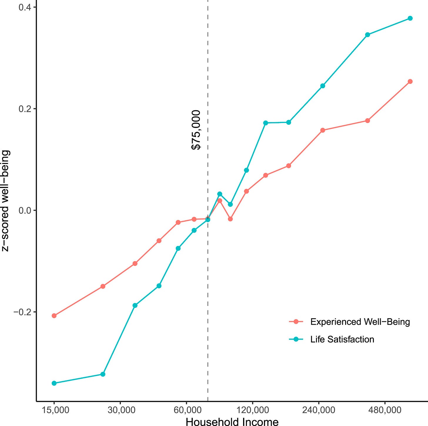
Happiness and income are related. A lot of research has established that. You can see this relationship play about both among individuals and across nations, and in both cases, it’s also clear that it’s linear in log(income).
Or in other words, the relationship between income and happiness is subject to diminishing returns.
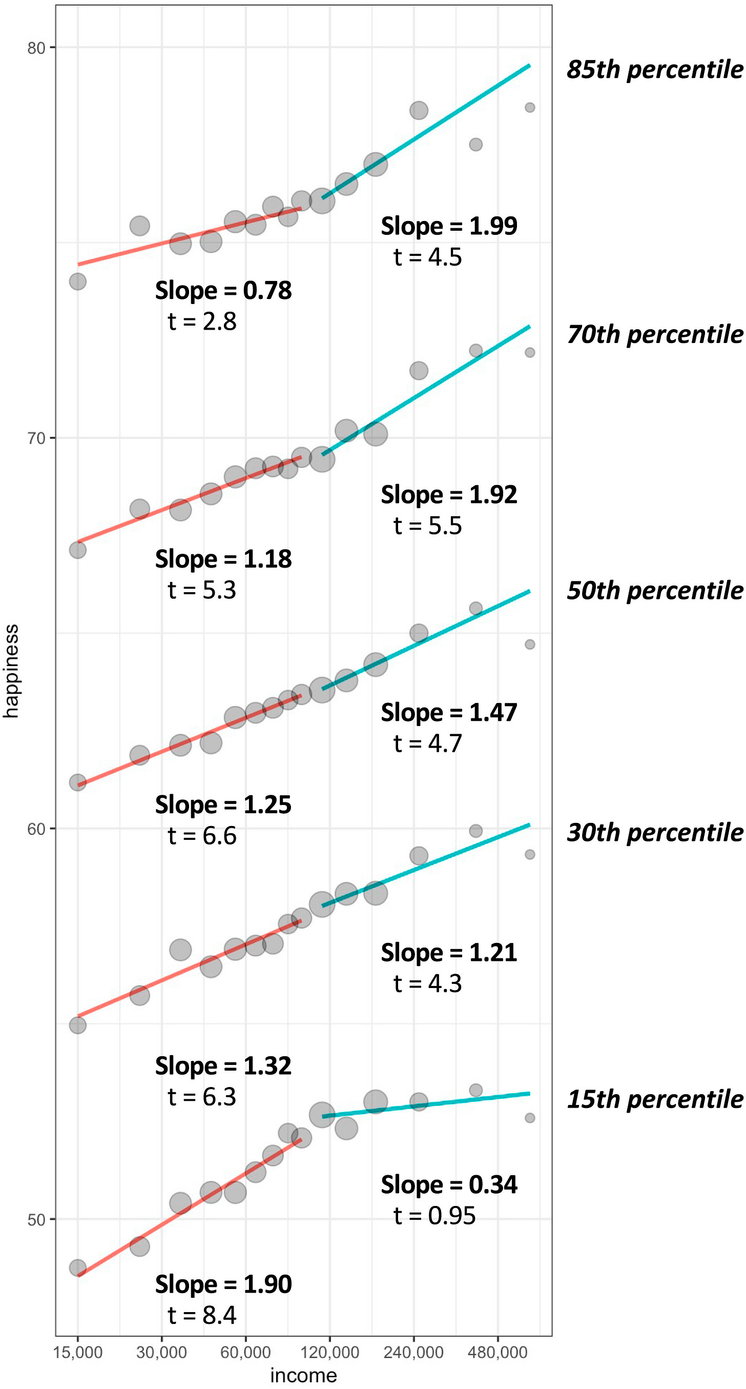
But two recent papers have disagreed about whether the relationship is linear in log(income). The first one found a relationship that was linear in log and it’s the source of the first graph. The second found that there were even more diminishing returns, such that they diminished in log(income) and not just income!
Like good scientists, the authors came together for an adversarial collaboration and they managed to reconcile their results: for very happy samples, there are increasing returns to happiness with higher income; for very sad samples, the relationship plateaus; for the 30th to 70th percentile of happiness, the relationship is pretty much linear.
These relationships are interesting, but it’s not clear what they mean. To assess whether this effect is causal requires going beyond side-eyed glances at the cross-sectional relationship and trends across countries. So it’s lucky we have a meta-analysis and systematic review of the causal evidence for an effect on the highly-related outcome of mental health.
But this systematic review revealed two unlucky things about the literature:
Most of the designs were low-quality and they relied largely on transfers, welfare, or changes in tax and wage policy.
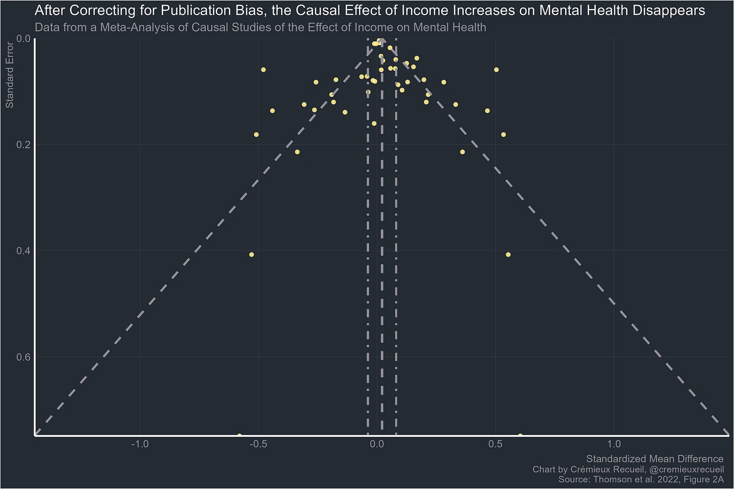
Their meta-analysis showed severe publication bias and the effects on mental health disappeared after correcting for it.
The issues with transfers and changes in tax and wage policy are highly notable. Firstly, the effects are generally small, so the resulting estimated effects are usually very noisy. Second, there’s often ascertainment and sampling bias. This is especially common when the welfare program has work requirements or we’re dealing with a tax credit that requires people to file their taxes and do so competently in order to receive it. It may be even worse when the proposed income effect happens through a resource windfall, like in the studies of local oil discovery effects in Norway. Third, proposed causal estimates from these studies usually greatly exceed the effect seen cross-sectionally and they are riddled with publication bias.1 Significant effects generally only appear after considerable conditioning, which usually makes it impossible to interpret what’s going on. Some studies even involve a nonlinear term that suggests that what’s being affected is something that’s actually measured differently at different levels of income, and thus we are sure that the estimate cannot be interpreted without serious psychometric modeling. This follows naturally from a lack of bias requiring equal effects at all levels of a measured psychological trait.
Let’s look at some of these studies from a domain that has more estimates available: income effects on IQ and achievement. Here’s most of the literature on welfare and antipoverty program effects:
Some estimates had to be omitted for clarity because they had SEs of 2.041, 2.720, and 1511.755. You may notice that the effects are driven by publication bias. If you include the extreme effects, you get that tautologically, but if you throw them out, you still get the same conclusion. In aggregate, there is no significant effect; after correction for publication bias, there’s really no effect. And it’s hard to expect anything different when the estimand for these is not actually very clearly an income effect on children’s achievement. We have more supposedly causal estimates, so let’s keep going.
In this paper, Tominey estimated a structural model to decompose household income shocks into either permanent or transitory components and then to estimate the effects of those on children’s achievement. But wait! We get diminishing returns again: lower income families show smaller effects of shocks on children’s achievement. This is intuitively sensible, but when you see this sort of nonlinearity, you must ensure that the measurements at different income levels are comparable. It would be far better to get comparable estimates if you’re interested in actually helping kids cognitively develop; if you are just interested in scores net of any effect on students’ ability levels, then this is actually fine. But the estimates are overstated because the identification method doesn’t actually satisfy the exogeneity requirement. These shocks are not necessarily random and, as is implied by nonlinear effects by initial income level, neither are their effects. Imagine someone earns a higher salary because they worked harder. It’s not clear that permanent income shock is exogenous.
So what’s the instrument and what’s the outcome? No one really knows, but the effect has to be overestimated, because it omits most people for whom the shocks available to be modeled were excluded for being too small. I would like this redone as a sibling control study in a register dataset without the major sample omissions this study had, but there would be a Flynn effect confound if that were the case.
Let’s keep going, we’re almost to the really good part.
This study exploited oil shocks and claimed a strong need to decompose heterogeneous marginals to even identify effects. But as noted above, doing that is psychometrically uninterpretable. That’s fine if you care about scores themselves rather than things like kids’ developmental or future attainment outcomes. But since the IV effect here is not actually exogenous—note: the income effect of the oil boom was not very large for initially low-income families, so the large nonlinear effect is contained among low-income opt-ins, who may systematically differ from low-income non-opt-ins—we can thus really only trust the fixed effects estimate that gives us the effect between siblings. But then we’re stuck with an effect that is not significant and if there’s anything there, it may have been driven by the Flynn effect.
My posts are long and you don’t have to read them all, but if you’re interested in this topic, there’ll be plenty here. Continuing: Canadian child tax benefit expansions.
This IV is not exogenous for the same reasons noted above. It also doesn’t deliver significant results, and the proposed heterogeneity by sex and age feels more like p-hacking than discovering something of substance. A sibling control should have been done, and it is possible with this data. So, noting that the power is really poor, I did redo it. Controlling for age, the within-pair effects are -0.05 for the PPVT and 0.06 for mathematics for the full sibling sample, both not significant. There was no interaction by sibling pair sex or for opposite-sex siblings. But again, there wasn’t much power. Using a more powerful and less causally-informative method, exploiting the multiple measurements, there’s also no significant effect down the line from benefits receipt.
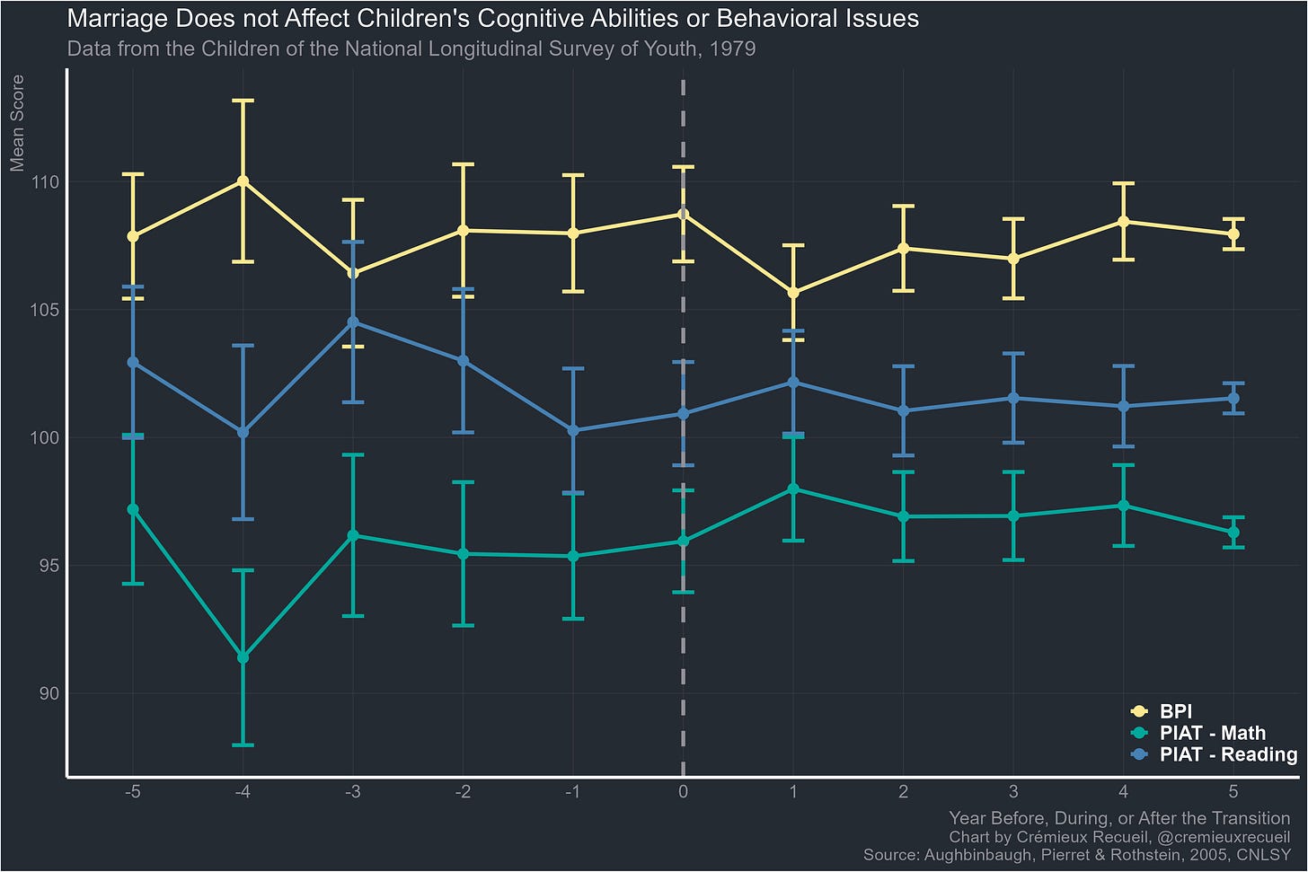
What’s another method? Well, we could exploit the fact that divorces and marriages have negative and positive effects on socioeconomic status (SES), respectively. Using the same dataset as Milligan & Stabile, here’s that for divorces:
And marriages:
Looks like nothing, consistent with natural disaster studies and studies of parental loss via accidents, both of which are in literatures that are rife with publication bias, and in both cases come with estimates that are often not exogenous because of endogeneity with respect to who is involved in accidents and who lives in zones that are vulnerable to natural disaster.
What about extreme event studies? There are several available, but documentation is generally not great. First, consider Holocaust survivors.

The “not great” part of the documentation here is thanks to the possibility of a survivor bias. Perhaps the smartest people survived, and also seemed to get PTSD. So a more understandable example is the Dutch Hunger Winter. There’s a lot here, so just read this thread on it. It delivered a more understandable null result through sibling control results.
What about moving people to well-off neighborhoods? This area of research is controversial because of very large selection effects related to opting in to programs like Moving to Opportunity. But here are the available estimates anyway:
So here’s a final method: adoption studies. These are life-changing. You get an entirely new family from an adoption study, and they tend to have high SES, very few psychiatric problems, minimal criminal records, and so on and so forth. What do they show? At best, small effects, and perhaps the importance of genetic confounding. For example, in the classic adoption studies by Caprom & Duyme, the SES of a person’s biological family was related to their performance, Black-White differences, g-loadings, etc. But adoptive family SES was not.
And this replicates! Here’s data from the Adolescent Brain Cognitive Development study:
Here’s the National Longitudinal Study of Adolescent Health:
Here are the Texas and Colorado Adoption Projects:
The Sibling Interaction and Behavior Study:

Skodak & Skeels’ adoptees:
The Swedish Adoption/Twin Study of Aging:

And finally, Swedish register data that shows no adoptee SES-performance relationship, higher scores for Korean as opposed to non-Korean adoptees or native Swedes, alongside a lack of selection effect confounding since parents could not select their Korean adoptees thanks to the law in South Korea.
And here are links to some other, mostly older, and all very noisy estimates/studies. For a very recent estimate, Willoughby et al. (2021) used adopted-apart kids to estimate that comprehensively improving the adoptive environment by 1 SD would lead to an increase in IQ of approximately 2.83 points, or about 0.20 d.
But we’ve gotten away from the point. What is the effect of income? Most designs aren’t really applicable for answering this question, but among those in the happiness-income meta-analysis, there were some valid ones. These were lottery studies. Lotteries offer large, varied, and pure income effects that are plausibly random with respect to winners.
We have large-sample estimates of the effects of income and wealth on both IQ and happiness. The way to assess whether the effect is causal with these studies is to compare the general population relationships with the ones found among lottery winners. Here’s IQ first:
In the general population, wealth is moderately positively related to IQs, good personality traits, GPAs, and scores in specific subject tests. Among lottery winners, whose wealth is uncorrelated with their traits, the same is not true: there is essentially no relationship between income and IQ or any of those other measurements. The implied causality is a confounded one. People who earn higher incomes have smarter kids for reasons other than the higher incomes. Perhaps they spend those higher incomes better than people who randomly obtain their money. We don’t know, but on its own, it is clear that wealth isn’t a cause of intelligence.
What about for happiness?
This is unclear! Earned and lottery income relationships with happiness, life satisfaction, etc. differ in precision and the observed magnitude differences for earned/lottery income effects aren’t significant for any estimate. Two of the estimates of lottery effects are not significant on their own, but it’s not clear what that means since they don’t differ from the cross-sectional effects either.
So we are at a causal impasse. But was there an effect anyway? Maybe, but this study doesn’t support it because the effects were driven by publication bias. Consider the effects of binary income increases on mental health:
And what about a binary decrease in income?
And if we’re just interested in continuous change?
There’s just not much here. Given that none of the studies in the review measured happiness properly to assess whether changes were real or just differences in how people interpreted the instruments, the literature actually seems pretty dismal: mostly weak designs, lots of publication bias, and not a single study took measurement seriously. Unlike with test scores, this isn’t a domain where that can be a passing concern because the score itself can matter either. If there’s an increase in a mental health or happiness score because of psychometric bias but people didn’t become mentally healthier or happier, that change was worthless with respect to intervention evaluation.
Incarceration Almost Certainly Reduces Violent Crime
This police chief is probably correct. At the very least, his stats are not wrong, and they’re also true for the majority of victims. This is an important point because victim-offender overlap speaks to the causes of homicides.
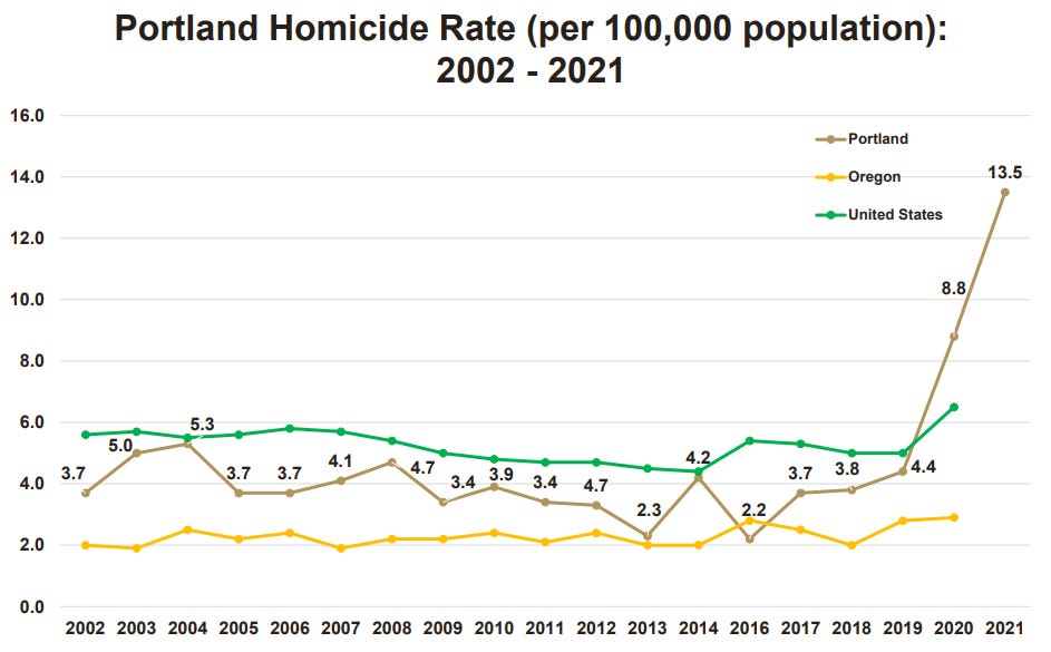
And a similar result holds in many other cities, like Portland, Oregon:
The Bureau of Justice Statistics recently provided some stats that show something similar: people who get sent to state prisons have an incredible number of priors arrests.
Another datapoint that is important here is that incarceration and homicides are negatively correlated:
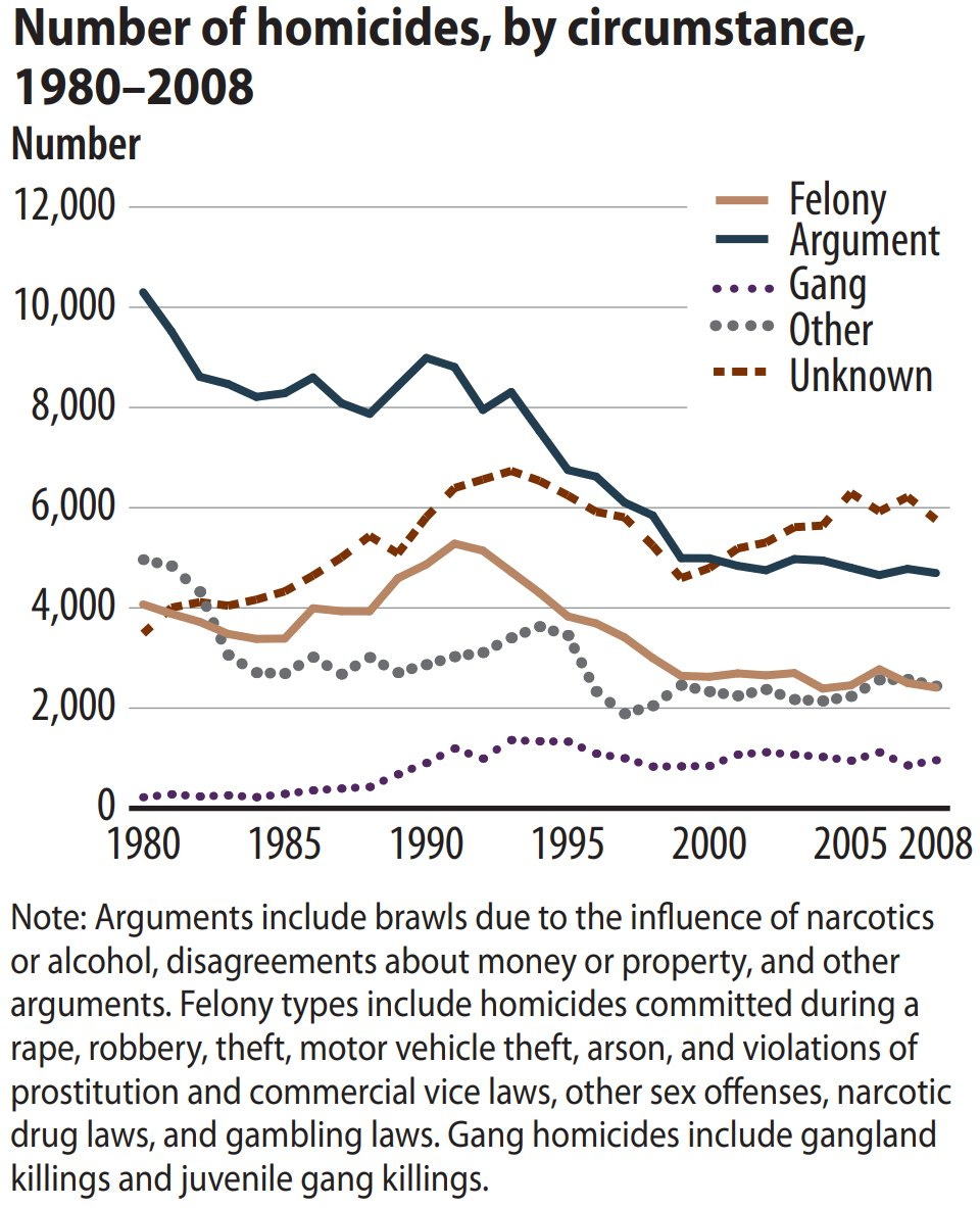
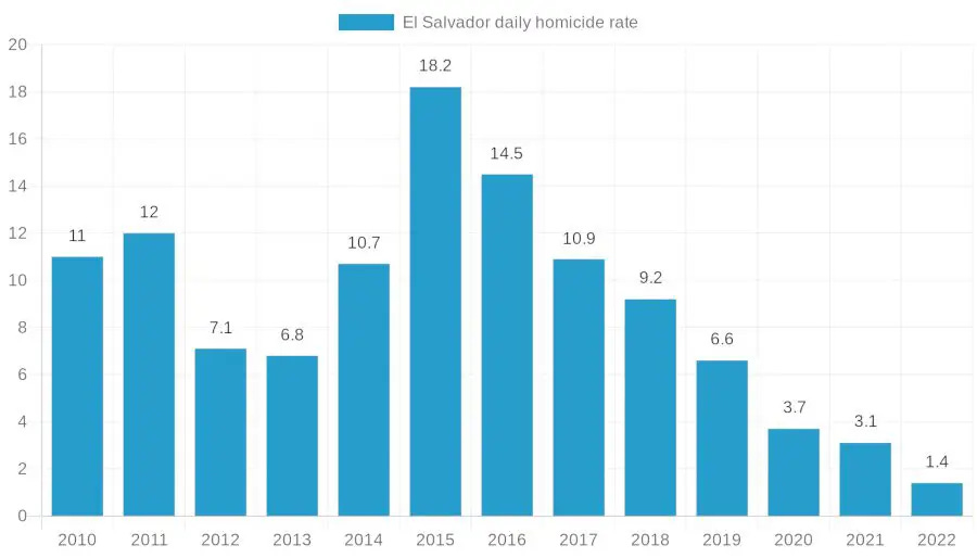
The conclusion that follows from this observation is basically unavoidable: if you lock up criminals, crime will go down. Most violent crime is not something that produces power vacuums. If a murderer gets locked up, another person will not step up to become a murderer. It’s not even gangs that tend to drive homicides outside of exceptional places like El Salvador.
And we know that shutting down gangs drastically reduces crime local to gangs, implying even other gangs won’t or can’t “step in” to fill in the violence gap left by gang elimination.
Because most violent crime is done by a small number of people, you only have to lock up a small percentage of people to achieve incredible improvements in public safety.
And it doesn’t take a genius to figure out who to lock up. You know what predicts committing a murder? Having previously committed a murder. And this applies to most priors, because criminality is a very a general thing: the man who commits an assault is also disproportionately likely to be the man to commit a murder.
The proof that this works can go the other way, too. All we have to do is look at what depolicing does. For example, after George Floyd’s death, people stopped cooperating with the police: the number of calls per gunshot fell immediately! And the effect of this went beyond the effect of the COVID national emergency.
And for clarity, yes, the decline in calls per shot also came with a decline in calls per casualty:
In another study, other prominent deaths were used to identify depolicing effects. They found that after events like Eric Garner’s or Michael Brown’s deaths, self-initiated policing and arrest activity plummeted, and they tended to fall more where there were more Black people.
And the post-Floyd depolicing effect on homicides seems to have basically only cropped up in places where there was a large movement to depolice. There’s a reason Portland saw a larger spike in homicides than Oregon as a whole.
A final note: Nayib Bukele is in the news recently for his work reducing homicide rates by arresting gang members. By all accounts, the measures seem to be working and El Salvador is on track for its least criminally violent year ever.
The reason this round of gang crackdowns has worked is simple: it’s the biggest round in history, and Bukele’s government hasn’t given up on it yet.
I’ve been looking for somewhere to slide this in. This paper argued that stopping criminals over many generations was responsible for Western European homicide rates declining: by executing and otherwise reducing the fertility of the most violent people, they managed to “breed out” violence and change the landscape of violence. And what a landscape it was!
The Gerontocracy
America’s Congress is now the oldest it’s ever been:


