Unlocking a Taxpayer-Funded Dataset

I digitized and modernized the National Collaborative Perinatal Project so that anyone can use it

I love open data. I love public data. I love data, and I want more of it to be available, especially when you’re entitled to access it by virtue of being an American whose tax dollars paid for the data to be created. For that reason, I’ve modernized the National Collaborative Perinatal Project (NCPP)—one of America’s premiere cohort studies.

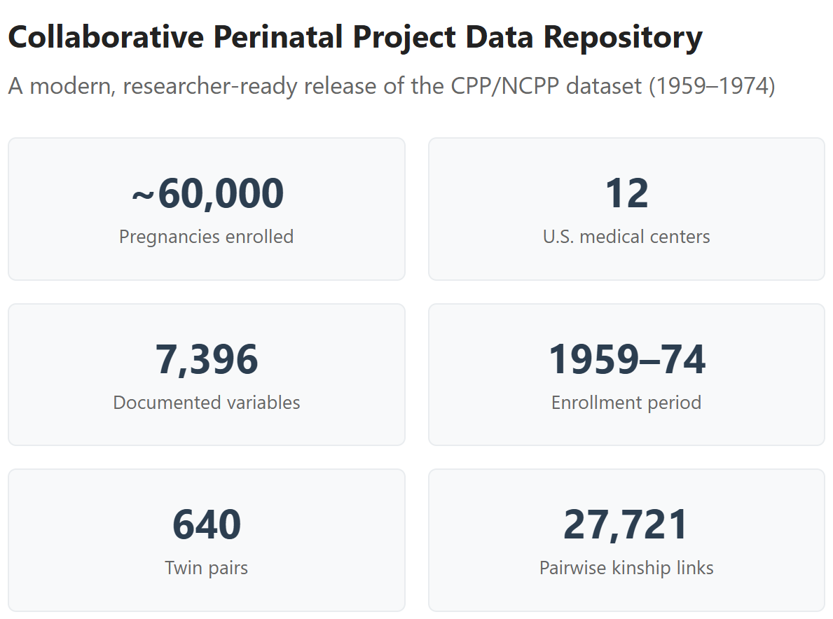
The NCPP is a huge dataset involving 60,000 pregnancies that happened across twelve U.S. medical centers between 1959 and 1974, with kids followed up for seven years, and measured across thousands of variables, from birth defects to growth trajectories to blood groups to IQs and personalities. Out there somewhere, subsets of the participants have been followed up for decades, but more on that later.

The big problem is that, for some reason, this meticulously gathered dataset that cost taxpayers millions to generate has produced barely any publications. Why? Simple: it’s a complete mess. If you want to access this wealth of data, you have to put in a lot of effort scanning microfiche. Microfiche is so old that most of you don’t even know what it is. Basically, it’s these tiny little slots of 10x15 cm transparent film containing highly reduced, unreadable images of documents, like newspapers, reports, and court and medical records. If you want to access that data, you have to scan that in, and that’s a lot of work!

So, with the help of our handy-dandy artificially intelligent assistant, Mr. Claude, I developed a scan and OCR pipeline that—with unfortunately large amounts of involved work on my part—eventually got all of the available NCPP data digitized. Then, I organized it, about 60% by hand, and 40% by Claude (if he’d errored less, he could’ve done more. Alas…), and made a website where you can search through all the variables, download all the data, and tell me if there are any problems that I might’ve missed.

From the website

As an added bonus, I’ve even expanded the dataset! (And I have more extensions planned.) Before I get onto showing you some of the really cool analyses you can run with this data, I want to tell you about those extensions. Want to skip that? Click here.

---

Dataset Extensions

I precomputed a lot of variables to make life easier for analysts who want to use this data. I provided g factor scores, growth measures, developmental and behavioral scores, and attrition and Census survey weights, but the big value-add is that I provided kinship links.

Kinship links are means of identifying siblings in the dataset. When you have siblings, this opens up lots of new analyses. For example, we can look compare siblings who were breastfed to ones who were not and see who’s more likely to develop allergies, a high BMI, a high IQ, or whatever else we might be interested in. With siblings who are different degrees of relatedness, like half-siblings (Relatedness = 0.25) versus full-siblings (R = 0.50), you can also fit behavior genetic models. Combine that with variables like sex and race and you can compute between-group heritabilities.

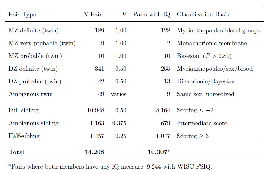
I constructed the kinship links in a few ways. For twins, I used determinations based on the ABO, Rh, MNSs, Kell, Duffy, Kidd, P, Lewis, and Lutheran blood groups, extracted from cord blood around birth. This allowed me to take the hundreds of twins—siblings born at the same time—and classify them as either dizygotic (fraternal) or monozygotic (identical) twins. But I didn’t have this data for every twin, so I used the twins I had and used other criteria and even built a Bayesian classifier to disambiguate even more of them.

For the non-twin siblings, I classified full- and half-siblings by way of a scoring system that integrates different types of evidence. For example, if a child’s father is listed as someone different from the father for their sibling, that’s a big bump towards ‘half-sibling’. One of the ways I thought I’d be able to distinguish a few half- from full-siblings was to use ABO blood groups for the mother and the children separately, to identify pairs where it was impossible for a given father’s genotype to produce both kids in a set. Unfortunately, this didn’t lead to anything substantive, but in fact, to identifying impossible combinations where the results for the kids couldn’t have even come from the mother. This meant identifying a very low rate of serological error, which was to be expected from the lab equipment of the time.

My sample ended up substantial, making this a great resource for future studies involving sibling and even cousin controls:¹

Table 6 from the data paper

Want to know what else I brought to this dataset? Go check out the paper!

---

What Can We Learn With This?

A lot! I have a short paper with some interesting tests over here. I’ll provide a few examples from it. Hopefully this piques your interest and you check out the paper.

General Intelligence is Real

How do we know if general intelligence—g—is real? There are several ways of getting at this question, but one of the most direct is a simple statistical test. This test involves comparing two models: a Common Pathway and an Independent Pathway model. Here’s an illustration of the difference:

Franić et al. 2013, Figure 1. On the left, a Common Pathway model; on the right, an Independent Pathway model.

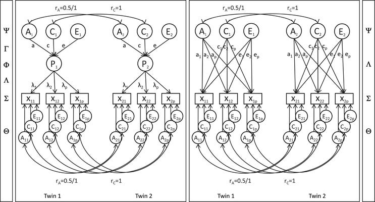
If you’re unfamiliar with behavior genetic models, this might look like strange esoterica. Basically, what this shows is estimating the heritability and shared environmental influence on some set of correlated indicator variables, X_1 through X_p. If the variables are correlated because of a latent trait like g, then the additive genetic (A), shared environmental (C), and nonshared environmental (E) influences on the variables run through the latent trait given as P in the diagram. This is a test of whether our understanding of a given construct actually carves nature at the joints, and if the test supports a given latent construct, then it’s much more likely to be real.

Several papers have tested this for a huge number of psychological variables, from personality to intelligence. In the domain of intelligence, the first explicit test affirmed a common pathway model—supporting g—in a Japanese sample. The second explicit test also affirmed a common pathway model, but in a larger study of American veterans. The third explicit test was by me—I found two common pathways and one independent pathway on a gifted sample, which might be explained by Spearman’s Law of Diminishing Returns—, but the third one that was published was done on a Serbian sample, and it supposedly found evidence for an independent pathway model. However, that model was misfit because one of the tests was a very unreliable measure (something I was able to show empirically on a much larger American sample!).² Finally, there’s a recent common vs. independent pathway modeling study, but it doesn’t actually test these models, it just uses the same words and runs some polygenic score analyses.

But enough about earlier results. I ran these model tests again for the NCPP. The independent pathway model fit best, but what this means is not totally clear because the independent pathway model was so similar to the common pathway model and the phenotypic g factor model.

The congruence coefficients between the A, C, and E loadings from the independent pathway model and the common pathway model come out to 0.995—essential equality—0.810, and 0.840, respectively—high, but not so high as to be identical. Thus, the genetic factor approximates the general factor. Moreover, a combined, vectorized congruence coefficient comes out as 0.911, and variance-weighted, it’s 0.952. The subspace overlap is 0.994 and the implied common variance—for the common pathway model, that means g—congruence coefficient is 0.995 and the rank-1 SVD share is 89.6%, versus a baseline of 68-83%. The common factor share of total variance attributed in the common pathway model is 57.8% versus 60.9% in the independent pathway.

The points of disagreement between the models had to do with the shared environment. By leveraging the independent pathway model, we can see that the shared environment is important for verbal and academic tests (Vocabulary, Comprehension) beyond what you’d expect from the variance directly attributable to g. In other words, the family’s environment affects those tests beyond g, but together, so they end up making the model with just g fit poorly. Perhaps this is why, when people find support for a common pathway, they tend to have dropped the shared environment, or used a sample where the shared environment is no longer expected to be involved due to the Wilson effect, where heritability rises with age, displacing it.

What these results end up telling us is that there’s considerable construct support for g: it appears to be very strongly linked to genetic influence, and not as much to environmental influence. But the model fits acceptably well, it’s just that there’s some subtest-level nuance that precludes it being the best option.

Note: The tests I ran were simple; I plan to come back and test additional factor configurations in the future, so there may still be a common pathway model that’s preferred over the independent pathway model. What I’ve shown is preliminary, but still highly informative because, given the dimensionality of the battery, all well-fitting results will converge, and every conclusion you reach with one model will be much like what you would with any other valid model. To that end…

Gene-Environment Interactions Don’t Matter for g

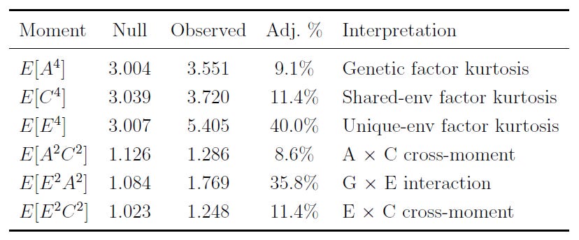
Even if the independent pathway model weren’t the ‘correct’ model, it can still be highly useful for several reasons. One such reason is that if it fits well enough, it sets us up to do powerful decompositions of the common and total variance across our tests, with implications for the common pathway model given how close to equivalent they are.

One of the things you can do is test whether the A, C, and E factors are actually interactive, rather than representations of additive effects. What this means is that you can determine the extent to which, for example, gene-environment interactions matter in aggregate as an explanation of particular factors, variables, etc. The result of checking this is… nothing! There’s next-to-zero evidence for interactivity, so the interpretation of aggregate genetic and environmental effects as acting additively is strongly supported, so non-additivity is not a worry for us.

Calibrated fourth-order moment tests for G x E interaction

Race Differences in IQ Are Heritable

Another cool thing the independent pathway model can do is it can be used to compute the genetic and environmental contributions to group differences. The common pathway model normally can’t be identified to allow this, and doing so involves more complexity than you get in a traditional ACE model.

The ability to do these decompositions was noticed back in 1989, but few people every ran with this. Since the advent of this method, only a handful of papers have used it, with a focus on the Black-White IQ gap in one, a focus on sex differences in alcohol use in another, and a focus on sex differences in conservatism in another. There may be a few more out there that I’m not aware of.

In any case, I’ve applied the same methods here, to the Black-White IQ gap. This table will be hard to read, so I’ll interpret it for you below.

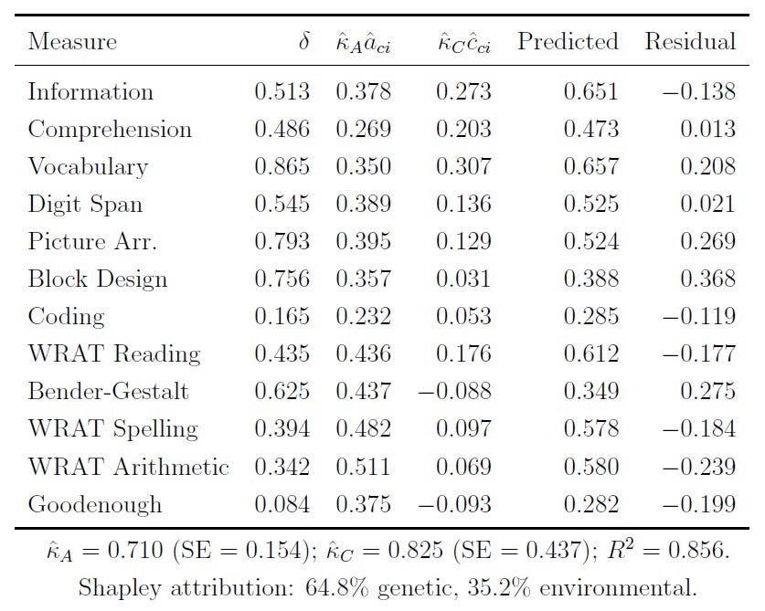
Basically, when we decompose the Black-White IQ gap, we see that the gap can be attributed to about 50% genetic and 50% environmental influence among these seven-year-olds. This is the gap in the common variance. When we include the variance specific to indicators, and not shared among them, the share of the gap that’s genetic rises to 55.3%.

This is not the be-all-end-all, as there was some minor measurement non-invariance in this battery: the loading for the Bender-Gestalt test and the intercept for the Goodenough test had to be freed to estimate the gap without bias. The effect of this is tiny, however, and the total genetic share of the gap rises just to 60.1%, with the common genetic share rising to 53.9%. Simply refitting the model without said noninvariant subtests delivers roughly the same result, with a total gap that’s 53.4% genetic.

That too is not the be-all-end-all, either, as there’s also the possibility that assortative mating—which has gone unmodeled—has inflated the shared environmental share relative to the genetic one, since it makes siblings more genetically similar than chance. Modeling values for assortative mating between 0 and 0.61 alongside our measurement invariance corrections, the common variance genetic share rises from 53.9% to 67.9% at a parental correlation of r = 0.20, and it goes to 96.5% at a parental correlation of r = 0.55. The total share rises from 60.1% to 83.7% at the same time.

The true estimate of the genetic contribution to the Black-White gap at this age (note: the shared environment fades into adulthood, so the genetic contribution will presumably rise) will likely be in-between the measurement invariance-corrected baseline estimate and the one with a parental correlation of 0.55. This gap, which we know to be highly genetic, is about 1 d (1.05 SDs) in size at the level of latent g, and a bit smaller at the observed level, which contains non-g variance and error variance.

People Can Personally Gauge Intelligence

When the WISC IQ test is administered, it’s done so by an examiner who listens to the verbal remarks of the child. In this dataset, the examiner also provides their subjective impressions of the each child’s cognitive function, personality, etc. The latent factor from these impressions is strongly correlated with latent g (r ≈ 0.9) and, as it turns out, these impressions are also entirely unbiased by race and they’re 90% as large as the tested Black-White IQ gap.

This might seem a bit boring, after all, the examiner generating the impressions just gave the child an IQ test. However, these impressions are not just tautological. They also correlate highly with a different, shorter set of tests that have objective scoring criteria independent of the examiner’s impression, and they correlate highly with test scores from a few years prior, when the kids were examined by someone totally different as four-year-olds:

Latent correlations among cognitive factors from four measurements

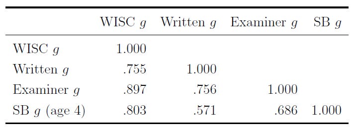
What the examiner sees is intelligence, as it’s measured. They can pick up on the positive manifold to a strong enough degree that their impressions from testing someone still manage to correlate about as well with different IQ tests as those IQ tests do with one another. That might seem simple and boring, but it’s incredible!

Brain Size Causes Higher Intelligence, Mediates Race Differences in IQ

In 1994, Arthur Jensen and his colleague Fred Johnson used this dataset to reach some interesting conclusions about brain size, intelligence, and race differences therein. To validate my findings and theirs, I’ve replicated their result and expanded on it.

People with larger brains tend to be smarter. This relationship is known to be causal. In the NCPP, the correlation between head circumference and IQ holds up for Whites and Blacks, and after adjusting for height and weight:

Sex-adjusted correlations between head circumference and WISC FSIQs

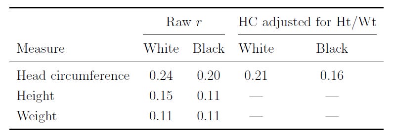
This association holds up within families, although it’s significantly attenuated. Between families, where family-level variables might inflate the association, the relationship is r = 0.272 with WISC FSIQ; within families, comparing siblings of all types, the association is still significant, at r = 0.098 and 0.107 for just the full siblings. (This association grows with age and goes higher with better-quality tests.)

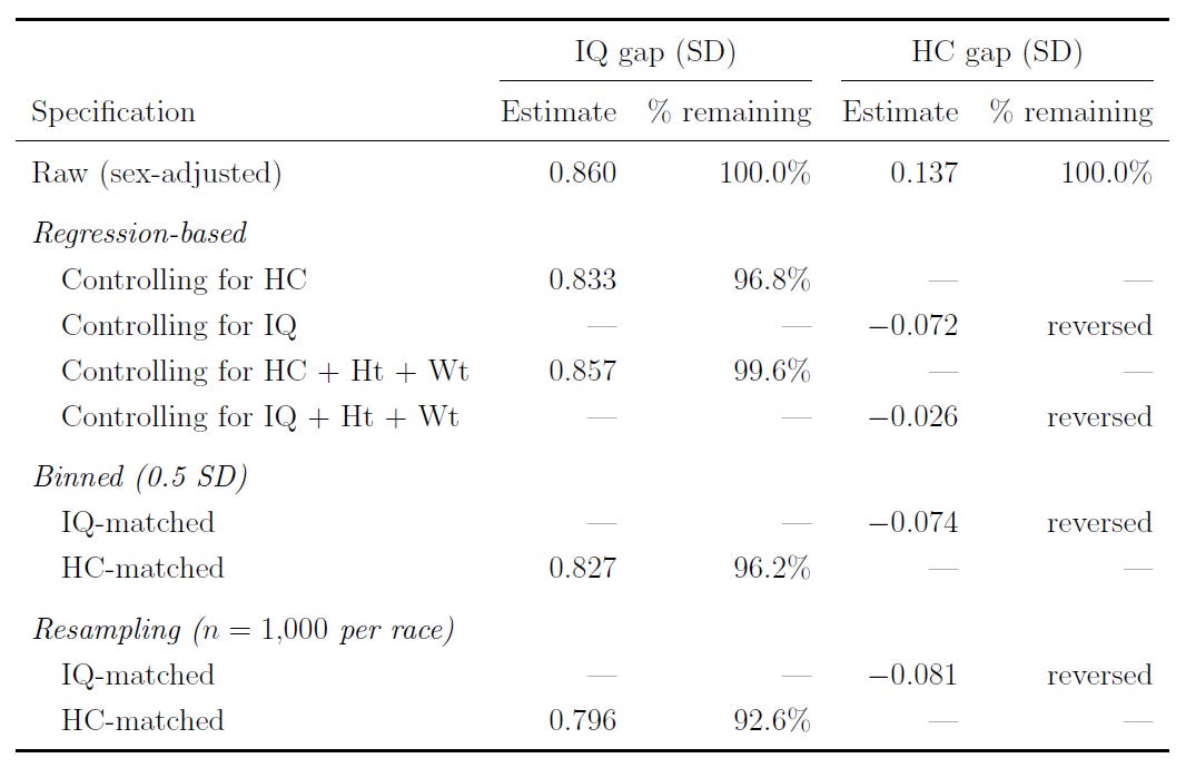
One of the really interesting things that Jensen showed was a practical demonstration of the phenomenon of' ‘supervenience’, or many-to-oneness. The way he did this was by showing that, if you control for brain size, the Black-White IQ gap only slightly shrinks. However, if you control for IQ, the Black-White brain size gap goes away. Raw brain size is one of many factors driving the IQ gap; IQ fully explains the brain size gap, as well as the gap in many other variables. Jensen only tested this with one form of matching, but I’ve extended this to several, all confirming the same result:

Controlling for head circumference leaves the IQ gap behind. Controlling for IQ eliminates the head size gap.

Another extension that I undertook was to look into whether any of the tests given to this sample predicted head circumference after taking out g. The answer between families, within families, and using multiple methods including just residualizing for factor scores or testing within a structural equation model was conclusive: at most, there are incredibly meager brain size-performance associations beyond g:

[Head circumference’s] entire association with the cognitive battery operates through g; there is no residual spatial or visual-processing specificity.

Since I’d recently seen people arguing that because males have larger brains than females on average and thus they must also have higher IQs, I decided to test that proposition, too. I found that when girls and boys were matched on IQ, girls still tended to have smaller heads. Given that, you might expect this next result: when they were matched on head size, girls tended to have higher IQs! And for thoroughness, I also found that when matched on weight and height, the slopes relating IQ to brain size were the same in both sexes.

Breastfeeding Doesn’t Affect IQ Scores

Even if breastfeeding didn’t help kids’ health at all, it would still be positively associated with all sorts of wonderful things and negatively associated with all the bad things in the world. The reason for this is that people today ‘know’ that breastfeeding is good, and the people who disproportionately adopt good habits are those who are well-off. Accordingly, their kids will tend to be well-off as well, regardless of the causal impacts of breastfeeding.

To get over this, we have to leverage natural experiments, randomized controlled trials, and within-family tests, where breastfed kids are compared to their bottle-fed siblings. The NCPP offers perhaps the most informative test of this to date, because when the NCPP began, breastfeeding was considered the unhealthy, low-class option. That’s just what people thought at the time, for whatever reason, so as a result, you can see things like 94.5% of mothers with <9 years of education breastfeeding versus 74.5% of college-educated mothers. You can also see that breastfed children averaged -0.65 SD lower WISC FSIQs—that’s almost 10 IQ points!

But, does that mean breastfeeding is actually bad? Well, let’s see. If we control for various maternal socioeconomic status variables, we can’t eliminate this negative association, only reduce it. Adding controls for birth weight, gestational age, smoking, and parity as well as a suite of neonatal health controls also doesn’t eliminate the association. So, naïve social scientists would likely say ‘yes, breastfeeding appears to be harmful.’ However, when we compare siblings who were breastfed to ones who were not, the association evaporates completely:

The bivariate cross-sectional association is large and negative: breastfed children score −0.65 SD lower in WISC FSIQ. Adjusting for demographics reduces this to −0.23 SD; full adjustment yields −0.15 SD. Under mother fixed effects, the coefficient flips sign: b = +0.08 (SE = 0.05, p > 0.1). All five IQ outcomes tell the same story—fully adjusted OLS associations are modest (WISC FSIQ: b = −0.15; VIQ: −0.02; PIQ: +0.05; SB IQ: −0.20; PCA g: +0.01) and all five FE estimates are small and non-significant (b = −0.02 to +0.13, all p > 0.05). The entire cross-sectional association is confounding from the reversed SES-breastfeeding gradient of the era.

This is one of the few times this has been tested. There are not that many within-family tests of the association between breastfeeding and IQ, so this is a big addition, not just because it’s another test, but because it shows that even in an era when the confounding was reversed, we can still back out the correct answer: a null effect!³

Socioeconomic Status and IQ

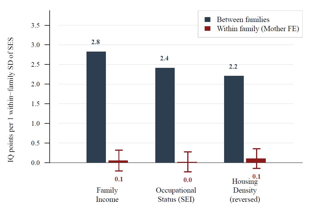
Within families, there’s exploitable variation in socioeconomic status that we can leverage to see if things like family income actually affect rather than just reflect ability. By using this, we can see that these variables have much small effects on IQ than is suggested cross-sectionally. That is to say, being in a wealthy family doesn’t matter that much for IQ:⁴

Figure 7 in the analysis paper

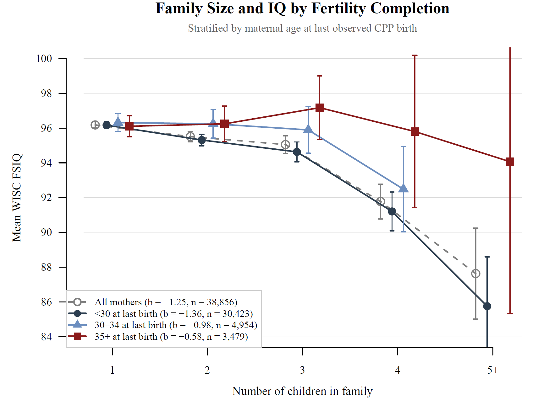
Similarly, I was able to run a variety of tests to see if the family size-IQ association was causal. Normally, this association is negative and strong, but it turns out it’s actually driven by confounding and family size does not predict lower IQs once that’s accounted for. I ran a lot of tests for this, but I’ll show you just one here: I found that among older mothers, a larger family was not related to kids having lower IQs. It was only among the youngest mothers—who are selected for being Black, poor, less educated, and having husbands who are similar—where a large family was associated with a lower IQ. That suggests a selection-driven finding!

Figure 4 in the analysis paper

A Peaty Non-Finding

I also tested something riffing on Ray Peat’s work. Ray Peat suggested papers born from mothers who had gestational diabetes would have larger brains. I checked this and, between mothers, the association was positive and nonsignificant (b = 0.03, p = 0.57), and it was still nonsignificant within families (b = 0.045, p = 0.88). There was nothing to do with IQ or effects at other ages or when stratifying by race either.

---

Have My Data, Have My Code

Everything I’ve done here is publicly verifiable. You have my data and you have my code; I’ve put it all online for you to see, to run, to critique, and to iterate on. It is yours, just cite my paper on the dataset if you plan to do anything with it. Doing so is a condition of using the data and/or the scripts I’ve provided, or for building from said data or scripts in any way. That’s not a big ask, so please, just do it, alright? Like so:

Lasker, J. (2026). The Collaborative Perinatal Project: A Modern Data Release.
OSF Preprints. https://osf.io/4tna9

I hope that more people will follow my example; I hope they’ll make their data and their code available to more people, and we can all come together and improve the scientific enterprise in the process. With that said, I hope you all appreciate what I’ve done here by modernizing the wonderful National Collaborative Perinatal Project!

---

Want to Help?

So, as I mentioned earlier, there are follow-ups for some of the participants in this data. These follow-ups go for various lengths of time, and unfortunately, none of them are publicly available, but all of them should be. The follow-ups I’m aware of are:

• Pathways to Adulthood (Johns Hopkins): Janet Hardy and Sam Shapiro followed 2,694 members of the Baltimore cohort through age 27–33 (1992–94), plus their mothers (G1) and children (G3), creating a three-generation study. 82% of participants were located; 65% interviewed. Archived at ICPSR Study #2420.

• New England Family Study (Boston + Providence): Stephen Buka (Brown), Jill Goldstein, and Larry Seidman (Harvard) have followed 17,741 individuals born at the Boston and Providence sites from the 1980s through the present day, with over 4,000 still active. The study has produced landmark findings on schizophrenia risk, ADHD, and adult cardiovascular health.

• Philadelphia-Providence Intergenerational Study: Klebanoff et al. re-contacted 1,782 female CPP offspring from Philadelphia and Providence in 1987–91 to study intergenerational transmission of preterm birth and low birth weight.

• Minnesota CPP 2.0: Logan Spector and Julia Steinberger (University of Minnesota) are conducting an ongoing follow-up of the Minnesota site cohort (now in their late 50s–60s), linking childhood exposures to adult cancer, heart disease, and diabetes via medical records and cancer registries.

• NICHD Mortality Linkage: Edwina Yeung (NICHD) linked 44,174 NCPP mothers to the National Death Index through 2016, enabling research on associations between pregnancy complications and cause-specific mortality across the lifespan.

These follow-up datasets are not included in this release because they are held separately by the individual institutions and were never incorporated into the central NICHD public-use files. The Pathways to Adulthood data is available through ICPSR; for other follow-ups, you have to contact the individual sites directly. I’ve tried, to no avail. If anyone would like to do that on my behalf, you can contact me on here or on GitHub with the results and I will gladly add them to the data release in later versions.

1. Note: As I state in the paper on this, there is minimal selectivity to being IQ-tested. However, there is some, and it has a largely morbid origin.

There’s no selectivity by socioeconomic status (d = -0.03 for the socioeconomic index and 0.04 for education), gestational age at registration (d = 0.08), or sex (balanced). There is mild selectivity for birth weight (d = 0.33) and for the WISC, there’s some for having a prior Stanford-Binet (SB) IQ score available (d = 0.19). The low birth weight thing, which hits twins particularly hard because twins have lower birth weights, is due to death. Lower-weight kids are more likely to die before age 7.

There’s also site-level variation. Site 55 has only 25.8% WISC completion vs. site 45 at 80.7%. This reflects administrative differences and is not really selective with respect to persons. For race, “Oriental” (0.2% vs. 1.0%) and “Puerto Rican” (3.4% vs. 13.2%) have much lower follow-up rates (37% and 39%), but the Black and White groups are comparable.

IQ availability is partially driven by child survival and site-based administrative differences, not by socioeconomic status or cognitive selection. The survey weights I provided in the release are designed to correct for both. Applying them minimally alters the results in the analysis paper.

2. On the subject of that Serbian sample, we can actually use a bit of basic math to flip the interpretation of the result. Whereas the authors assumed—wrongly, given the unreliable WCST measure—that they had affirmed an independent pathway model, their common factor loading matrix (the loadings from A_C and E_C) suggest a common pathway is substantially correct. The way I flip the interpretation is through a singular value decomposition (SVD) of the common factor loading matrix from the study. You can obtain that from the authors’ diagram:

Nikolašević et al. 2020, Fig. 1

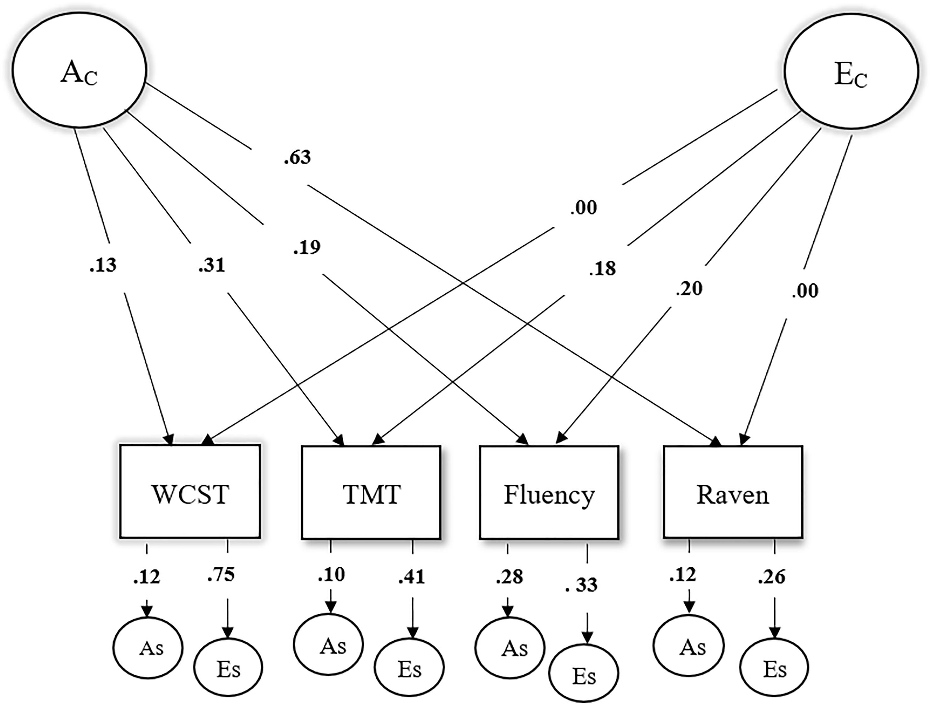
The first thing to note is that the model is obviously misspecified because there are some loadings that are exactly zero. The second thing to note is that an SVD suggests that 87.6% of the variance is rank-1, meaning that this data is about 90% compatible with proportionality, and thus something close to the common pathway model, there’s just a small 12.4% share that is not.

Quantitative qualification ought to be used whenever people are doing independent vs. common pathway modeling, because with a large sample size, less than total unidimensionality, and with measurement error, it is almost-certain that even when you have, say, 95% support for a common pathway, you’ll reject it in favor of the independent pathway model because large-enough samples practically ensure less parsimonious models will win.

However, the quantitative evidence should probably be better than just an SVD—which needs to be calibrated—and should include stuff like loading comparisons between models. Unfortunately, with just the data provided by Nikolašević et al., we’re not able to get that. But, I do go on to show how this can be done for the NCPP data in the supplementary materials.

I was inspired to do this by various GenomicSEM papers that have broken down the extent to which genetic effects on intelligence tests and other measures are consistent with affecting the general dimension (a la a Common Pathway) versus specific indicator variables (a la an Independent Pathway).

3. I will also not here, though I didn’t put it in the paper, that breastfeeding was negatively related to head circumference at birth (-0.36), 1 year (-0.24), and 7 years (-0.27) in OLS, even with adjustments (-0.32 to -0.20), and it was at best tenuously related within families (-0.21 at birth, p = 0.03; -0.01 at 1 year and 0.04 at 7 years).

4. For reference, the Black-White gap in socioeconomic status was 0.45 d for education, 0.96 d for occupational status, 0.72 d for family income, 0.57 d for housing density, and 0.62 d for a unit-weighted composite versus 0.82 d for a latent socioeconomic status composite—from a model that fits poorly—and 0.95 d for a first principal component factor score.