
GDP is Inevitable
GDP is a reviled metric, but it's still one of the best we have. I explain why mathematically.

This was a timed post. The way these work is that if it takes me more than one hour to complete the post, an applet that I made deletes everything I’ve written so far and I abandon the post. You can find my previous timed post here.

In 1938, the mathematician Samuel S. Wilks showed that the correlation between two composite variables will approach 1.00 when the component variables are positively correlated and the weights in the composites are all positive.1
To understand the practical implications of that statement, first, I’ll define what I’m talking about.
A composite is a sum of different variables. GDP is an example, as it’s built up from the combination of consumption expenditures, investment, government spending, and net exports, (C + I + G + NX). A test score is also a composite, as it’s the sum—weighted in some fashion—of a person’s scores on individual test items. Total factor productivity, the Global Innovation Index, the Better Life Index, Big Five personality scores, different depression indices—these are all composites too. Their component2 variables are just the things that are added together to make the composite.
Because Wilks was publishing in 1938, he didn’t write out a modern proof. I’m also not going to do that for a Substack post, so, let’s do something like that, albeit extremely simplified. Let’s establish a plausibility heuristic, and if you need a proper proof, go read the original paper.
Let x₁, x₂,…, xₙ be correlated variables with unit variance (i.e., SD = 1).3 We define two different ways of summing them up, using two different sets of weights, k and l, as follows:
If the average correlation between these variables is positive and the number of variables n grows towards infinity, the correlation between the sums converges to 1. To prove this, look at the correlation coefficient formula:
When we expand the covariance of these two sums, we get a matrix of every possible pair of variables. We can split this into the diagonal terms (where a variable correlates with itself) and the off-diagonal terms (where it correlates with another variable):
As n gets larger, the sums approach their expected values based on the average weights (a and b) and the average correlation (r̅):
We do the same for the variance of each individual sum. The variance of the first sum looks like:
Notice the difference in power. The first term—the unique variance—only grows linearly with n. The second term—the shared covariance—grows quadratically with n². When we plug these back into the correlation formula, the n² terms become so massive that they overwhelm the n terms. As n goes to infinity, the unique weights disappear from the equation:
Because the numerator and denominator are now identical, the result is 1. Thus:
This result is also extremely robust. In a 1996 paper from Krieger and Green, they found that the two assumptions of Wilks’ theorem—“positively correlated attributes and independent choices of weights”—were weak assumptions, and the convergence between composites holds up without “extreme, simultaneous violations of both assumptions”.
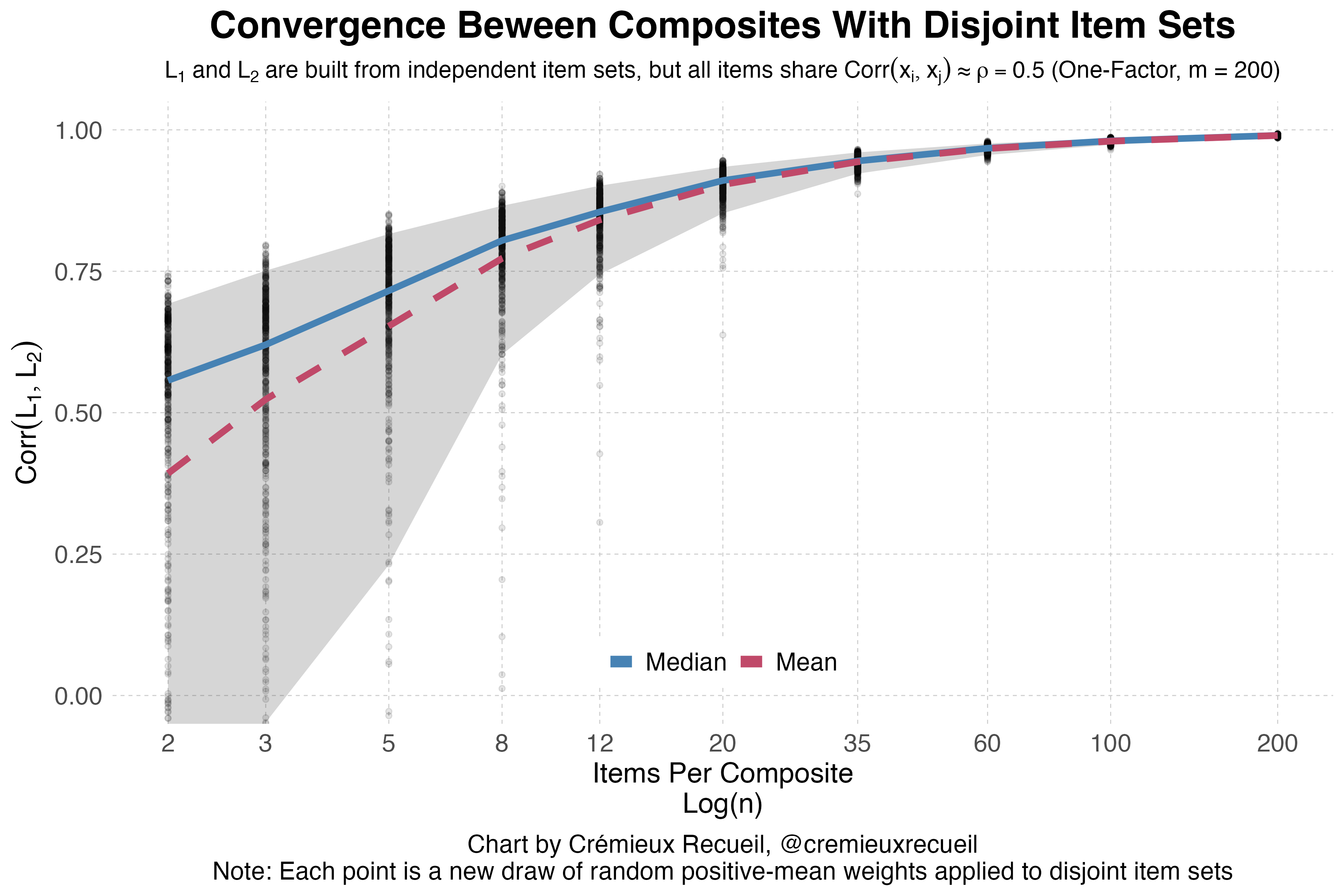
Visually, you can see these correlations rising rapidly even with disjoint sets of items whose intercorrelations that are, on average, quite modest, at around 0.5. If you adjust this upwards, the convergence rises faster, and if you adjust it downwards, it rises more slowly, but in both cases, it rises.
Thus, GDP
The practical impact of this is that it is almost inevitable that GDP will correlate with tons of things very highly, purely by virtue of its parts correlating with tons of other things found in different composites. Oftentimes, this is even more true than we might expect for another reason: that some of the things included in GDP are directly included in other things. Sometimes GDP itself is included in other composites, and, moreover, sometimes there are variables that are near-transformations of what’s in GDP that are included in other composites.
To add insult to injury, ecological measurement—measurement at a highly aggregated level, like the state or country—means that variables like GDP, when it’s credibly computed, should be highly reliable and have little unique variance: aggregation removes within-group variance while preserving between-group covariance. That means mechanically inflated correlations and is part of why you see things like individual-level IQ vs. income estimates of 0.3-0.4 versus country-level IQ vs. income estimates of 0.7-0.9.
There are strong mathematical drivers behind GDP’s correlations with other composites, and with many other variables that effectively index GDP, even when those things are not directly causally rolled up with GDP per se.4 That much is certain, so now I want to talk about some other implications of Wilks’ curious finding.
One implication of Wilks’ idea is that if you do something that should theoretically make a measurement more reliable for some purpose, you can make it less reliable for another. For example, if you make a healthcare quality index that includes lots of facets like healthcare expenditures, number of available hospital beds, and availability of new cancer drugs, then you could make something that is much more comprehensive and theoretically interesting, but as you add items, it becomes harder to distinguish from regular old GDP. It converges to GDP very rapidly, in fact.
This matters a lot in domains like psychology, which is what Wilks was concerned with. Consider the constructs of “grit” and “conscientiousness”. Is grit just a facet of conscientiousness? It’s highly correlated with conscientiousness, and it seems to slot in as a facet under the Big Five model. To make a better grit measurement, you’ll need more items touching on grit, but… as you add items, reliability will tend to increase, but our ability to distinguish the score from conscientiousness will decline. This is true unless you begin to define grit by items that are negatively correlated with conscientiousness, but somehow still remain correlated with the rest of grit. This is unrealistic based on current data, and if someone were to attempt it, it would bound the content of the items unreasonably.
This is also why it generally (but not always!) doesn’t matter what test you use to assess something like a group difference. The ecological issues I noted are why this tends to matter even less at higher levels of aggregation. That’s why, say, national IQ score differences so closely match national PISA score differences.
This is a big problem when there should be differences between constructs. GDP should not equal health quality, but for simple mathematical reasons, it does; IQ testing should not so closely match the results of an achievement test, but it does; grit isn’t exactly conscientiousness, not lexically or theoretically, but in practice, they’re unable to be distinguished.5
GDP is important, but keep Wilks (and aggregation phenomena) in mind when you attempt to justify it.
Or at least consistent in direction. If a negative value for an item on a test is a better performance, it’s consistent and not disruptive to weight it negatively, even though all the other items are weighted positively.
Not to be confused with principal components.
Let’s also take the law of large numbers for granted and ignore that I’m not mentioning independence, positive means, finite moments, r̅ > 0, and using proper convergence notation.
See, relatedly, the composite score extremity effect.
This is why I think sum scores may be psychometrics’ greatest achievement as well as its greatest failing.
"A composite is a sum of different variables. GDP is an example, as it’s built up from the combination of consumption expenditures, investment, government spending, and net exports, (C + I + G + NX)."
I am going to disagree with you on GDP. The United States' GDP relies heavily on the financial sector, which has little to do with a country's economic health or living standards. China's GDP relies more on actual production. There is no standard for what is and is not allowed in the variables. A great example is the comparison of the US GDP and China's. When using GDP as a proxy for average IQ, the United States shows an average IQ higher than China's. When tested IQs are compared, that is not the case.
https://www.smartcapitalmind.com/what-are-the-different-problems-with-gdp.htm
Thank you sir. This was fascinating as not a math guy myself. But how does your field account for Goodhearts law? I'm assuming there's some kind of formula to account for this. Even if it's just a manual scale down being taken from the positive perception bias data (is how I would do it heuristically). But it probably wouldn't work that well. If you have time, I'd love to learn more. Thank you!
Respectfully,
Staffing Weenie