
You Can't Just "Control" For Things
Statistical control usually doesn't make an analysis causal and it can easily mislead

This was a timed post. The way these work is that if it takes me more than two hours to complete the post, an applet that I made deletes everything I’ve written so far and I abandon the post. You can find my previous timed post here.

There is a common tendency to claim that an effect is causal after using a few control variables. This tendency is unfortunate because statistically controlling for things is rarely as simple as adding a few covariates to a regression. I’ll briefly explain.
Controls Require Causal Theories
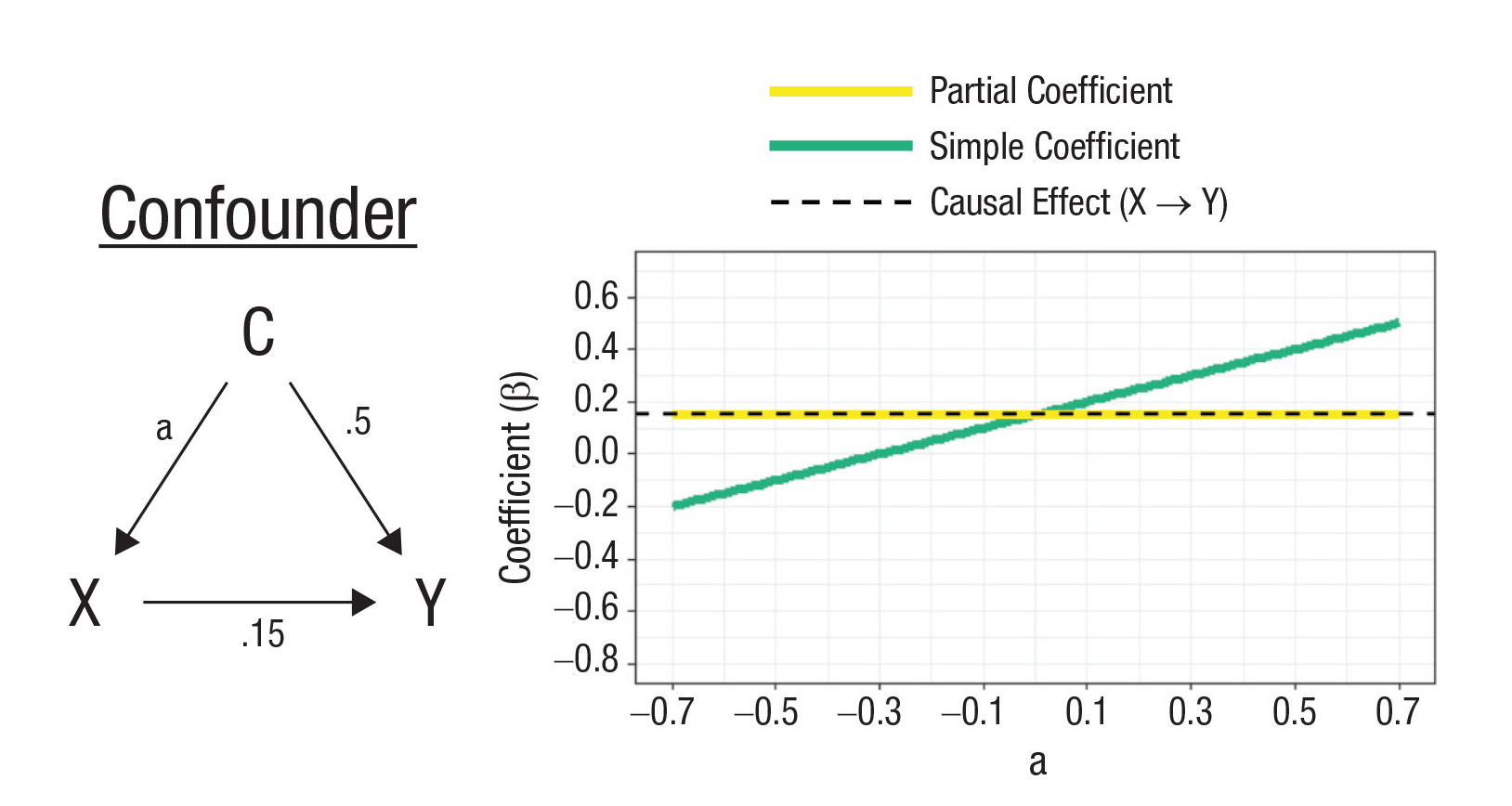
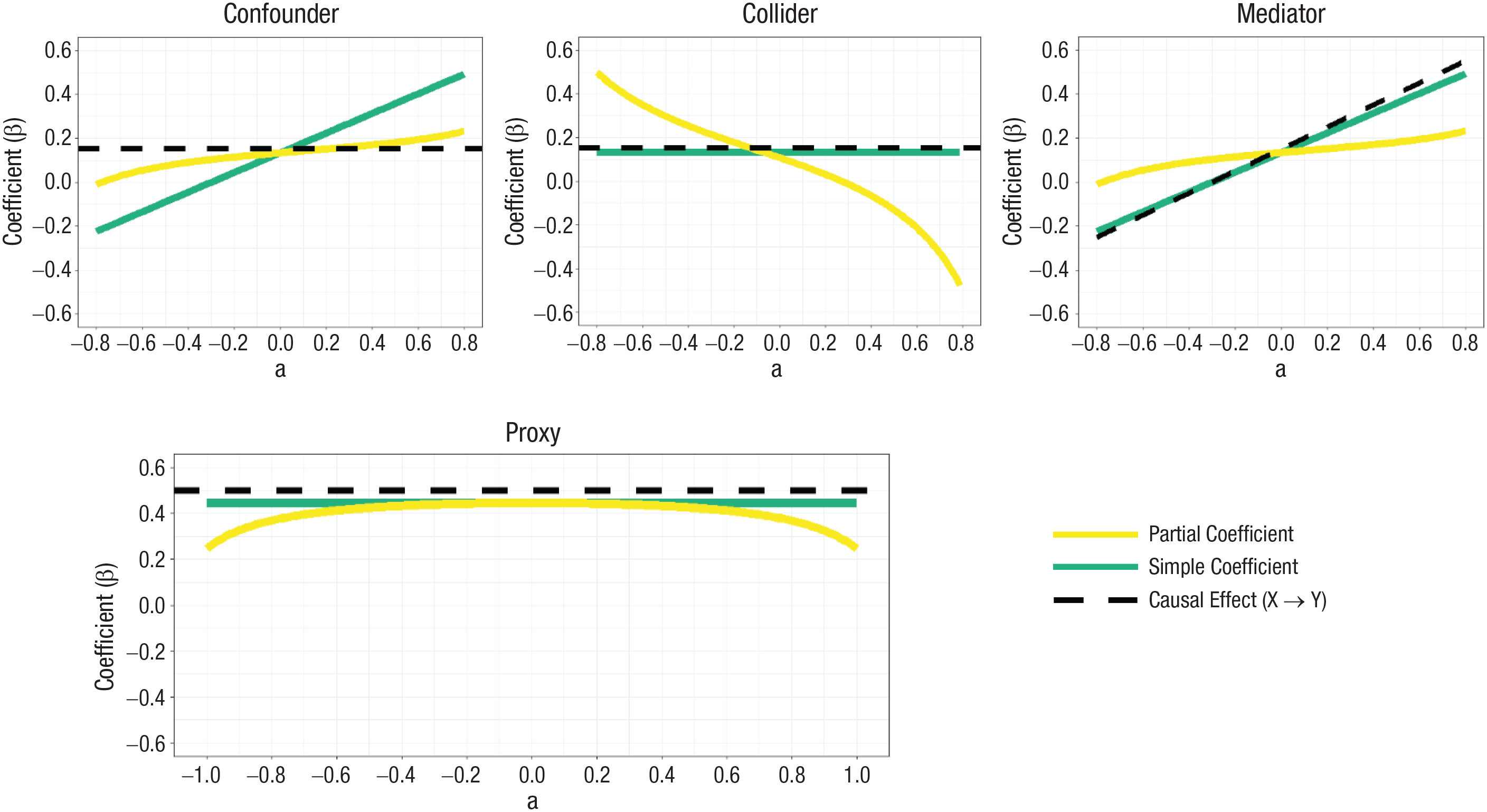
So you want to figure out whether and to what degree X causes Y. Unfortunately, there’s a confounder, C, in your way. C is a variable that causes both X and Y, linking the two beyond the direct effects of X on Y. That means regressing X on Y alone will not tell provide an answer to your questions. Fortunately, there are measurements of C available, and you can just control for it to remedy the issue. Do that, and you get the effect of X on Y—that is, the partial (i.e., conditional) coefficient matches the causal effect. In this simple case, controlling works.
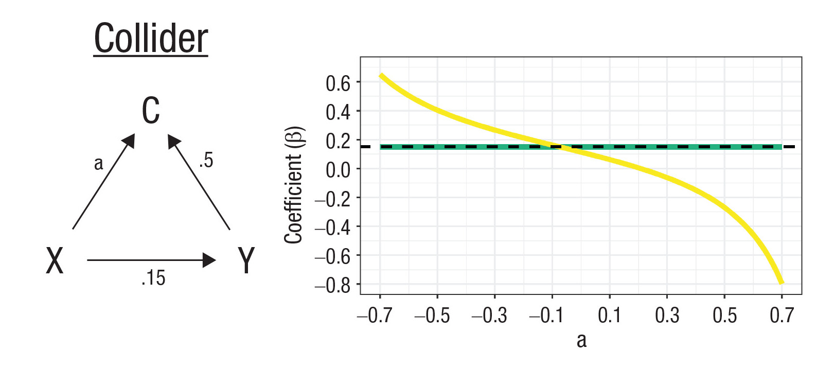
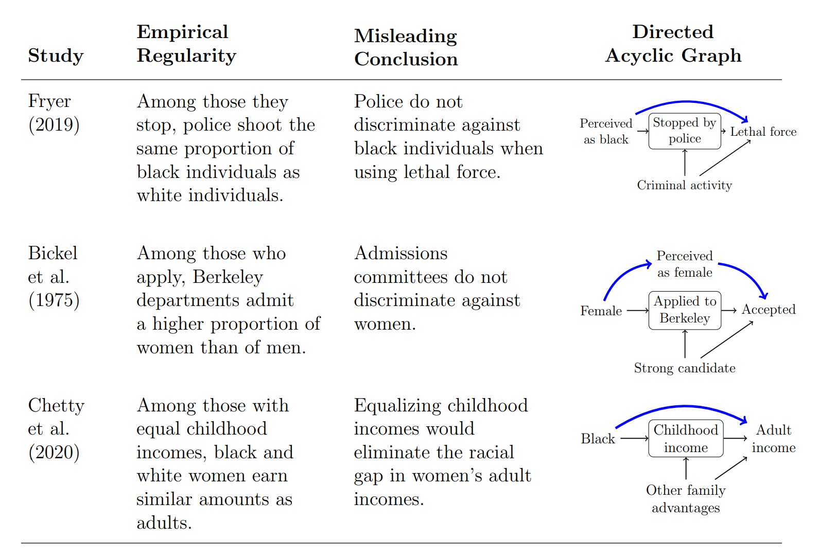
Let’s imagine the directed acyclic graph (DAG) on the left side of the diagram above changes. Now we’re dealing with another type of variable—the collider. Colliders differ from confounders in that the paths from C to X and Y are instead reversed and they now come from X and Y: C doesn’t cause a link between X and Y, but instead, a spurious link between X and Y shows up when C is controlled for.
One concrete example of a collider comes from the COVID pandemic: If age and infection are associated with opting into voluntary data collection efforts, they’ll be associated within the sample, even if they’re not associated in the general population the sample is drawn from. Or, imagine a scenario where you sample college students, and being conscientious and high-IQ both predict getting into college. In that sample, collider bias might generate a negative correlation between the two variables since they can compensate for one another in the selection process. Students who lack a high IQ might otherwise be highly conscientious and vice-versa. In this case, if you control for C, you’ve made a mistake.
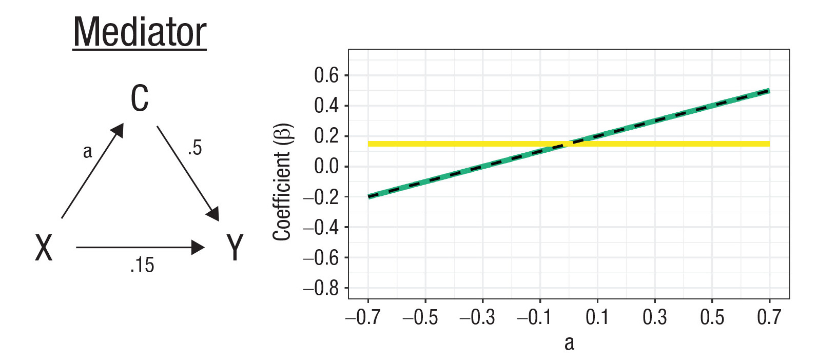
Let’s change the DAG again. Now C will be responsible for the connection between X and Y—it’ll be a mediator. C is caused by X and causes Y, in whole or in part. For example, depression may be related to tiredness because it leads to insomnia and sleep disturbances. Controlling for a mediator blocks off one of the paths between X and Y, distorting estimates of X’s total effect on Y, and can also lead to collider bias.
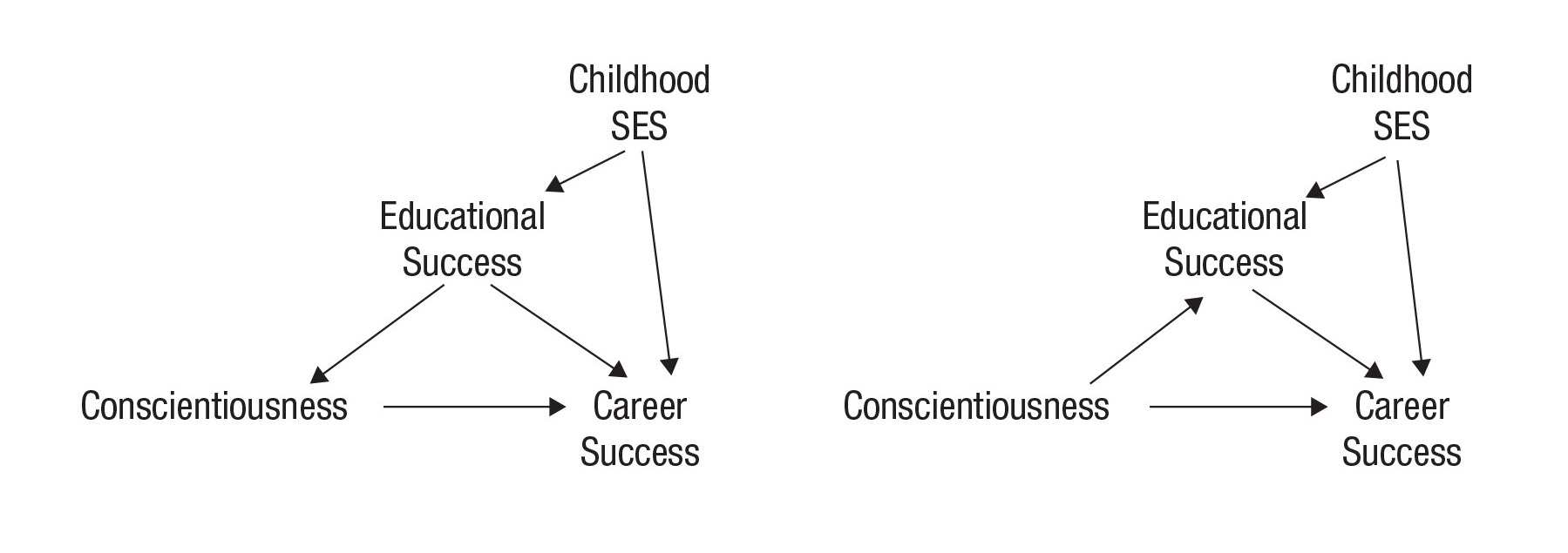
There are more types of variables, and far more complex DAGs than these, and the identities of different variables as colliders, mediators, or confounders in those graphs can be uncertain. For example, consider these DAGs of the relationship between conscientiousness and career success. One of these DAGs depicts educational success as a mediator, and another displays it as a confounder; what it really is can be difficult to ascertain, and getting it wrong can materially affect results. Even worse, it can be both. It’s not even clear that all of the paths shown are correct, as childhood socioeconomic status (SES) might also affect conscientiousness. Conscientiousness measured earlier in time—which is likely to be correlated with conscientiousness measured later because traits are often stable—could even influence childhood SES because a child with certain propensities might prompt their parents to work harder. Who’s to say?
To make this worse, controls are often not measured very well. For example, you might want to control for a personality measure that only has a reliability of 50%, or you might want to control for income, but it varies considerably for idiosyncratic reasons from year-to-year such that a single year’s data is an unreliable measure of a person’s attained living standards. If you were trying to figure out the effect of breastfeeding on a child’s intellectual development, it would make sense to control for a mother’s IQ, but this measure will come with some level of unreliability, and if the father’s IQ isn’t in the equation, there’ll be even more error approximating the child’s IQ and the effort to control will be incomplete.
Often enough, measures for X aren’t even just unreliable, they’re actually proxies for something else besides the theoretically correct X, and they can be more or less reliable in their role as proxies. In the best cases, proxies are just unreliable measures of what you really want to measure, as in the case of personality measurement. In worse cases, they’re different things and they might even have relationships with your variables of interest independent of the thing they’re supposed to proxy for. In other cases, C is a proxy for X, and controlling for it can cause a variety of issues. Even the random error in an 80% reliable X can have serious effects on your ability to obtain correct estimates of its effect on Y when you control for its highly-correlated proxy, C, as shown here:1
In short, controls have to be justified theoretically, or they may very well lead us to the wrong conclusions. Control for something causal, like a confounder, and you’re likely to be fine; control for something non-causal, like a collider, and you’re likely to end up wrong; control at all when the question is about the total effect of X on Y, and you might end up with an estimate of only part of the effect you want to estimate, or if you’re unlucky, you might end up with something totally different by doing that.2
Matching Is Usually Insufficient
Many studies attempt to estimate the causal effect of exposures by matching observed groups and then comparing them cross-sectionally, longitudinally, and so on. The idea is that, after matching their baselines, changes over time will be causally interpretable because they’re otherwise equivalent, so changes can be ascribed to an exposure.
The fatal problem for this method is “residual confounding”—when the set of variables used for matching is not broad enough and/or measured well enough to remove the effect of confounding. In some cases, residual confounding can be addressed with only a handful of controls, but such cases are rare. A more typical case is one where even large numbers of controls leave behind considerable confounding.
The most informative example of which I’m aware comes from a comparison of experimental—causal—and nonexperimental peer effects estimated in extremely large-scale Facebook data. Facebook randomly assigned millions of users to either see or not see stories about a peer sharing a URL and they estimated the effect of peer URL sharing on a person’s own likelihood of sharing said URL with a total sample of some 215 million observations. They then paired this with nonexperimental estimates of the same effect based on 660 million other observations.
The nonexperimental estimates were biased upwards by more than 300% without any adjustments. Even adjusting for demographics (age, gender) left behind a massively biased estimate. Adding in general behavioral variables, bias went down, but remained extremely high, even including more than 3,700 different measures of prior behavior. Using domain-shared rather than general measures led to more bias reduction, but still produced a relative risk estimate that was two-thirds of a unit higher observationally than in the experimental setup.
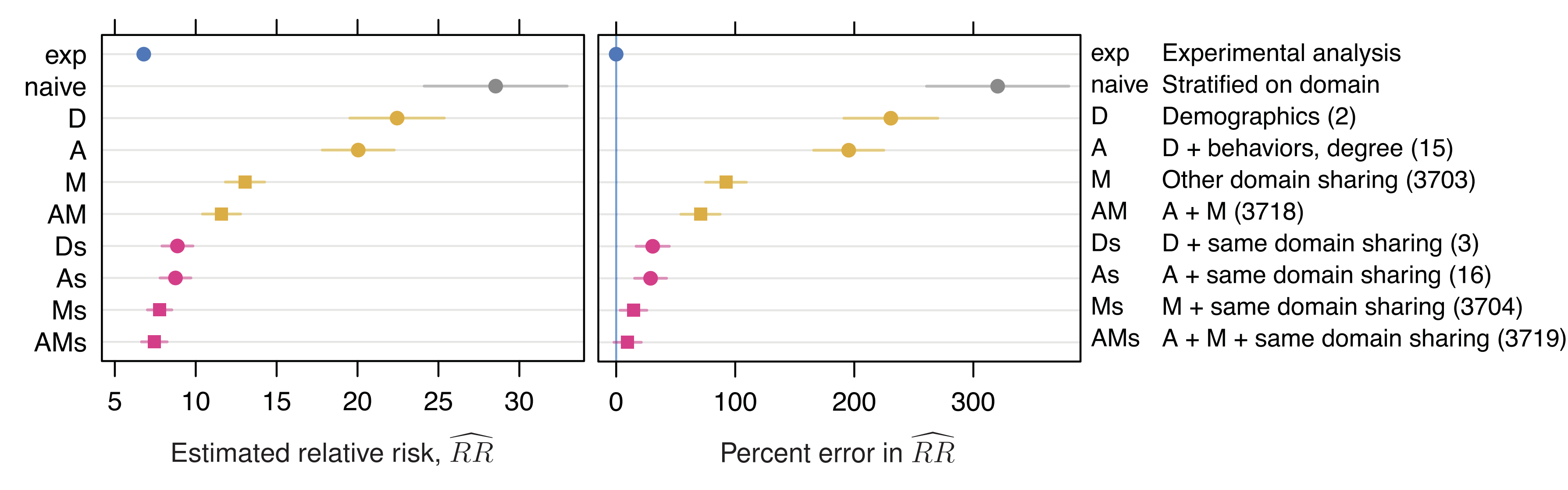
In this instance, matching was not sufficient to practically eliminate bias until about 3,700 different controls were in use. I can only hope this is more extreme than in the typical case, but regardless, it serves as a warning that it can take a lot of data to get rid of residual confounding. The data requirements can be so great that datasets may simply not support it, and estimates that are equivalent to experimental ones may be out of reach.3
Overcontrolling
Matching is good and all, but with other designs, it’s not usually what we mean by controlling. In those designs, researchers have to worry about controlling for too much. To see why, imagine two restaurants: any old McDonald’s and a featured Michelin 3-Star fine dining establishment. After we’ve controlled for the quality of ingredients, preparation, atmosphere, clientele, and price, the two cannot be (statistically) distinguished. So, you may conclude, they’re really not all that different. But you would conclude wrong, because you’ve controlled for too much and the comparison no longer makes sense.
The risk of overcontrolling can be made all the worse by small sample sizes. Computationally, without very large samples, it can be difficult to separate the effects of different variables. When different variables are collinear, their influences are even harder to distinguish, and controlling for them can lead to massive inflation of standard errors, computational problems, and outright nonsensical estimates of their effects.4 A famous example from a case where researchers attempted to estimate teacher value-added to students should suffice:
Some examples of what multicollinearity can do to coefficients can be seen by viewing the list of regression weights reported by Bingham et al. For example, a student who was older than average when attending second grade was expected to be 3.55 points above the fifth-grade grand mean, but a student older than average when attending fifth grade should score 7.40 points below the mean. Another example is that four variables reflecting students’ involvement in free lunch programs in Grades 2 through 5 had positive coefficients, but a summary variable reflecting involvement in the free lunch program had a compensatory negative coefficient of about the same magnitude as the sum of the coefficients for the 4 separate years. Another example is that missing data for an item pertaining to the number of schools the pupil attended in second grade had a negative coefficient, but missing data for estimating the mean number of schools per grade had a positive coefficient.5
Or, in other words, the issue with comparing McDonald’s and fine dining has a counterpart in interpreting variables controlling for many other variables. What’s a 3-Star restaurant net of the things that define a 3-Star restaurant? What’s “third-grade exceptional education” net of the things that define—or even merely correlate with, if we’re unlucky enough—an exceptional third-grade education? In these cases, the estimate and the estimand have come apart.
Designs and Identification Threats
One way to get around the need for controls to identify causality is to look for observational cross-sectional designs that theoretically remove confounding from the picture.
For example, why might wealth be associated with different political views? Estimating the cross-sectional effect of wealth by simply regressing it against different people’s views potentially leaves tons of confounding on the table because people who hold certain views have certain amounts of wealth and hold those views for nonrandom reasons. But if wealth is effectively randomized due to, say, winning the lottery, then that fixes things by severing the link that causes both wealth and political views in the general population. Data on quasi-experiments like that is available, and it suggests the cross-sectional ‘effect’ of wealth is, indeed, not much like the causal one.6

But, what if certain people with odd combinations of political views are disproportionately likely to partake in lotteries? And what if this is regionally-specific, and people who tend to win more or less in lotteries tend to have certain personalities, in certain regions? This is not even close to reality (and luckily, other designs like the twin one agree with the lottery estimates), but if it were the case, then the design might not be informative about our central question. There would be an identification threat—something that precludes the causal interpretation of an estimate.
Many designs for causal inference run into identification threats. For example, say you want to estimate the effects of Radio RTLM—sometimes referred to incorrectly as “Radio Rwanda”—on genocide perpetration during the Rwandan Genocide. If radios for listening were distributed nonrandomly, then that could make using their distribution in earlier years as an instrumental variable a poor instrument for Radio RTLM penetration and consumption. If the radios did not lead to Radio RTLM listening at all, then they would be a poor instrument for that reason. Developing a deep, qualitative understanding of Radio RTLM and its surrounding institutional environment actually does make it appear as though it cannot be a good instrument.
In some cases, instrumental variables used for the purposes of causal inference are so overused that they imply the instrument cannot be a good one for some case. The most popular example of this is rainfall. Rainfall has been used as an instrument to estimate the effects of so many different things, that those things it affects must be on the causal paths to many other variables rainfall affects and has been shown to affect, making causal inference with rainfall very difficult indeed.
In principle, any given observation can be explained in multiple ways. Whether a particular design for a study is causally informative depends on how many things can plausibly explain an observation. Identification really only takes place when the number of explanations is just one. Unfortunately, the options on the table can be too numerous even when the identification methods appear, at first glance, to be sufficient, leading to situations where interpretations can legitimately vary, and more work must be done to decide between them.
Even Experimental Controls Need Work
When all else fails, run an experiment. Randomize groups of people to different experimental conditions, and estimate the effects of those conditions. Ta-da! You have causal inference, you’ve overcome any issues you might’ve had with controls because you randomized, and you’re set to expound on your findings for the whole world.
Right?
Well, maybe. Your experiment could be broken. You might’ve needed blinding and failed to achieve it. You might’ve run the experiment incorrectly and not known it, or you might’ve paid for someone else to run it and they might’ve done it wrong without your knowing. You might’ve even been doing a survey experiment, and you might’ve ended up with a bunch of trolls, AI-generated responses, and so on. Even if you get to do a gold-standard randomized controlled trial, you still have to think about how it’s run.
Even assuming you do everything else right, you might not have used the right type of control group. This often happens when one group partakes in an intervention, and another group is left disengaged, doing nothing. In such a situation, the control group is passive. An active control group, on the other hand, would be exposed to an intervention of their own. This active intervention can be something simple and hopefully irrelevant. For example, you might have a treatment group given working memory training and an active control group that’s told to go play hide-and-seek.
This is not a merely theoretical concern. Giving people a placebo pill or a sham injection is a form of active control that can seemingly moderate effect sizes to a substantial degree7, or even affect retention in a sample. Compared to passive controls, the effect sizes from trials with active controls that are as simple as that are generally a bit smaller. Empirically, when people run IQ-boosting interventions with passive control groups, they tend to find substantial effect sizes. But when an active control group is used, effect sizes evaporate and estimates move towards zero and generally become nonsignificant.8

Sorry, But You Have To Use Your Brain!
Controls are not things you can use without thinking. You might think you know what to control for, and you might be wrong; researchers might think they know what to control for, and they might also be wrong. Unfortunately, when it comes to statistical control, simply plugging different covariates into a regression is not a shortcut to avoid hard thinking. If you want to reason scientifically, you’ll have to use your brain.
This is also related to the desire to justify using controls by way of their incremental validity. In a world where there’s measurement error, including more controls can just mean including more measures of the variance that’s due to something you’ve already measured.
A prominent example of this is so-called “grandparent effects” on social status. In many datasets, social status seems to be predicted not just by the social status of one’s parents, but also by their grandparents. But the reason grandparents appear to offer predictive power is simply because parents are being measured unreliably and grandparents are correlated in their traits with one’s parents. In these cases, the variance attributable to grandparents disappears when parents are measured very well.
Concluding that a control is not superfluous because it supplies incremental validity can easily be fraught like this. In the grandparent example, it has persuaded people that grandparents matter even in situations where they cannot, such as when they died young without bequests and lived very far away, long before modern communications technology, or when their kids—the parents—were adopted away. Gregory Clark has written about this.
And there is no shortcut to figure out what types of variables you’re working with. To make this clear, in the simple DAGs shown above, the correlation matrices can be identical!
The results also show that careful selection of covariates can help to reduce residual confounding more than haphazard selection. This echoes claims like those raised in the debate over whether experimental and matched estimates of the effects of work programs are equivalent.
Mean centering fails to obviate this issue.
This issue is a common motivation for using principal components or summary measures.
A related issue that this paper discusses is that people will often control for something and then conclude that the residual is explained by a particular variable. In the study critiqued in this paragraph, the authors concluded that, after controlling for a bunch of variables, the residual was the value-added effect of teachers. This is not an appropriate conclusion, because the number and/or variety of controls might’ve been insufficient or otherwise in error.
This issue frequently pops up when people control for polygenic scores and then conclude that the residual contains no genetic influence, even though polygenic scores are not complete indices of genetic influence. Another place this pops up is in estimating the size of the illegal immigrant population. To get at illegal immigrant numbers, people will adjust surveyed foreign-born numbers in various ways and then conclude that the illegal immigrant population is whatever is left over. This method only works coincidentally, if the assumptions—which are often wrong—are correct, or at least balanced in their errors.
This also suggests that twin estimates are very close to lottery estimates, meaning that they too can be used to remove confounding of this sort.
To be sure, I am still a skeptic of the placebo effect.
My suspicion is that this is because people lose interest if they’re not kept engaged. This study contains empirical evidence to that effect.
This is giving me epistemic vertigo
Thank you for writing this.
Rarely comment, but really appreciated this post and a digest of the work of Wysocki et al. (2022), which offers a well-articulated critique of statistical control and its limitations when divorced from causal justification. It echoes the foundational arguments made by Judea Pearl—particularly in The Book of Why—against the overreliance on control groups and purely statistical associations for causal inference. While control groups can reveal associations, they often fail to address hidden confounders and cannot, on their own, establish causality.
Pearl’s “ladder of causation” that encompasses associations, interventions, and counterfactual reasoning, emphasizes that causal understanding requires structured assumptions and formal tools. Causal diagrams (DAGs) and the back-door criterion provide a framework for identifying which variables must be adjusted for to estimate causal effects in observational data. Wysocki et al. effectively highlight this point [citing Pearl in 4 instances], cautioning against common missteps, such as adjusting for colliders or mediators, which can introduce bias or obscure causal pathways. Their discussion of proxy variables is similarly nuanced, recognizing both their potential and their pitfalls.
While the share post and discussion draws heavily from Wysocki et al., it’s essential to recognize the broader context: the sophistication of modern causal inference should enhance, not diminish, public trust in science. The complexity we confront in modeling causation is not a weakness—it’s a necessary response to the multifactorial, dynamic nature of biological systems. Scientific claims like “X causes Y” are appealing in their simplicity, but the real work lies in rigorously navigating a web of interdependent variables, mediators, confounders, and evolving biological processes.
Pearl, J., & Mackenzie, D. (2018). The book of why: The new science of cause and effect. Basic Books.