The Other Type of Flynn Effect

When we talk about the Flynn Effect, we need conceptual clarity

This was a timed post. The way these work is that if it takes me more than an hour to complete the post, an applet that I made deletes everything I’ve written so far and I abandon the post. You can find my previous timed post here.

---

I’ve read the entire literature on the Flynn effect. I’ve reanalyzed all there is to reanalyze, conducted novel analyses, reproduced and replicated results, and helped researchers with papers on the subject. My understanding of the Flynn effect is this:

Increases in scores across cohorts and decreases in scores across cohorts (so-called ‘anti-Flynn effects’ and ‘Woodley effects’ alike) are attributable to psychometric bias: measurement non-invariance that, when corrected, tends to moot or at least substantially reduce the scale of temporal trends. The psychometric location of the Flynn effect is primarily on those subtests with lower g-loadings, and there is usually a g-unrelated affinity for certain skills and group factors. The Flynn effect is primarily about test-taking sophistication and norm obsolescence.

This understanding is an accurate summation of the whole literature that I would challenge anyone to disagree with on empirical grounds. On that note, I know exactly how it could be challenged, and I want to explain why such a challenge is invalid.

There are a handful of studies that are allegedly studies of the Flynn effect (and some that are adjacent to it) which purport to show real, measurement invariant test score decreases and increases across various times and places. While most Flynn effect studies are driven by measurement bias, these other studies sometimes actually aren’t. These studies are instead driven by sampling bias.

---

An exemplary study that showed a positive Flynn effect is Ang, Rodgers and Wänström’s one in which they used the Children of the National Longitudinal Survey of Youth (CNLSY) cohort to showcase the Flynn effect in the PIAT Mathematics test. What they found was that five, six, seven, eight, nine, ten, eleven, twelve, and thirteen-year-olds’ scores trended up in each year of the survey data. The extent of these trends was similar by sex, race, and urbanicity, but children from more educated and higher-earning households showed a stronger Flynn effect—that is, greater score increases in successive years of the data.

So, in short, what they did is they looked at all the people who were a given age in a given year and, in later years, people of said ages tended to have higher scores.

Do you see the problem here?

If you don’t, that’s perfectly alright. None of the peer reviewers or editors at Intelligence or any other journal publishing similar analyses noticed the problem either. Once I say it, it’ll become a glaring problem and you might even notice it in other papers. I’ll give you another hint before coming out and telling you. Take a look at this chart that uses data from the same sample:

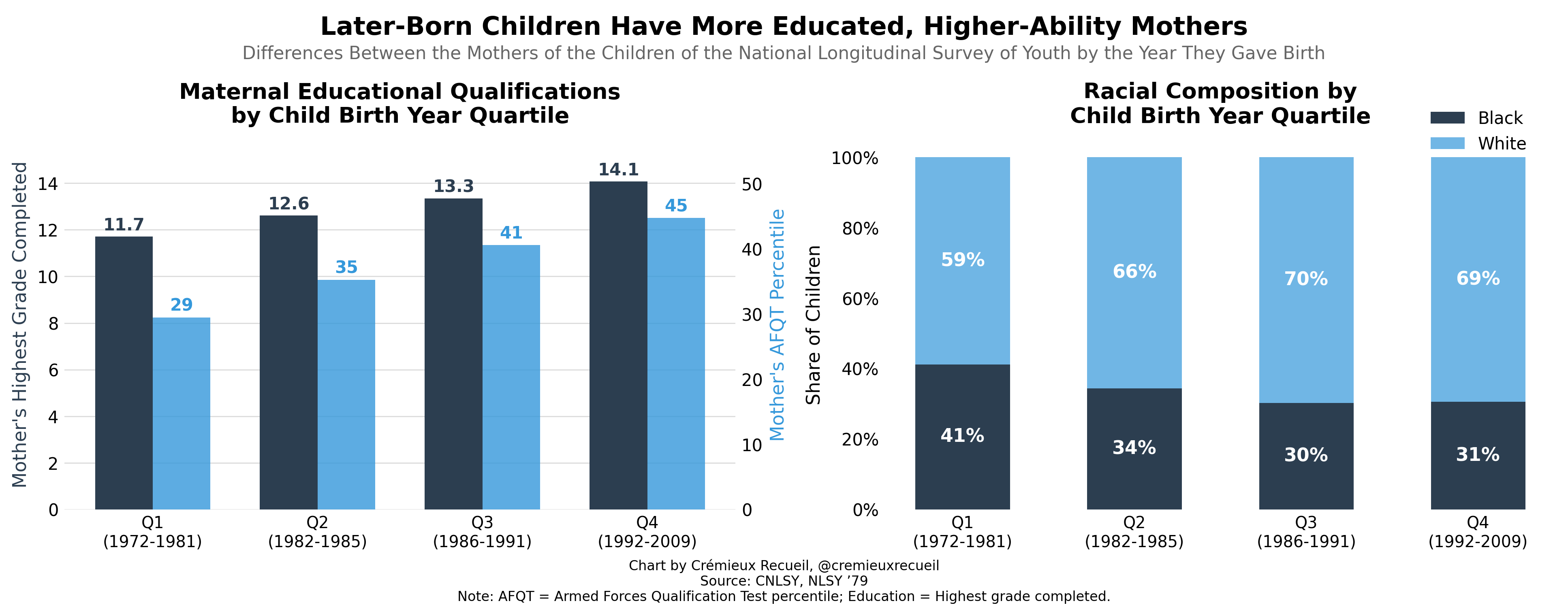
Children born later in the CNLSY sample had mothers who were (1) better educated; (2) smarter; (3) more likely to be White as opposed to Black. Ang, Rodgers and Wänström’s results are clearly confounded: smarter kids are born later because smarter people tend to have kids later! Fair to Ang, Rodgers and Wänström, they recognized this possibility and controlled for measures of mothers’ intelligence. But, they did not have measures of fathers’ intelligence and their measures have some degree of unreliability, so the control is likely not enough to remove all the residual confounding.

You Can't Just "Control" For Things

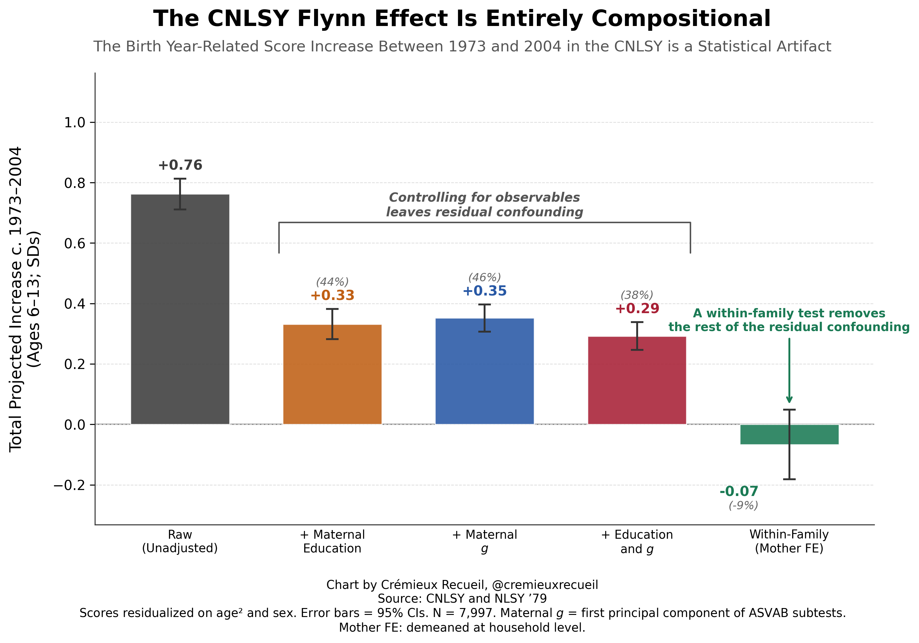
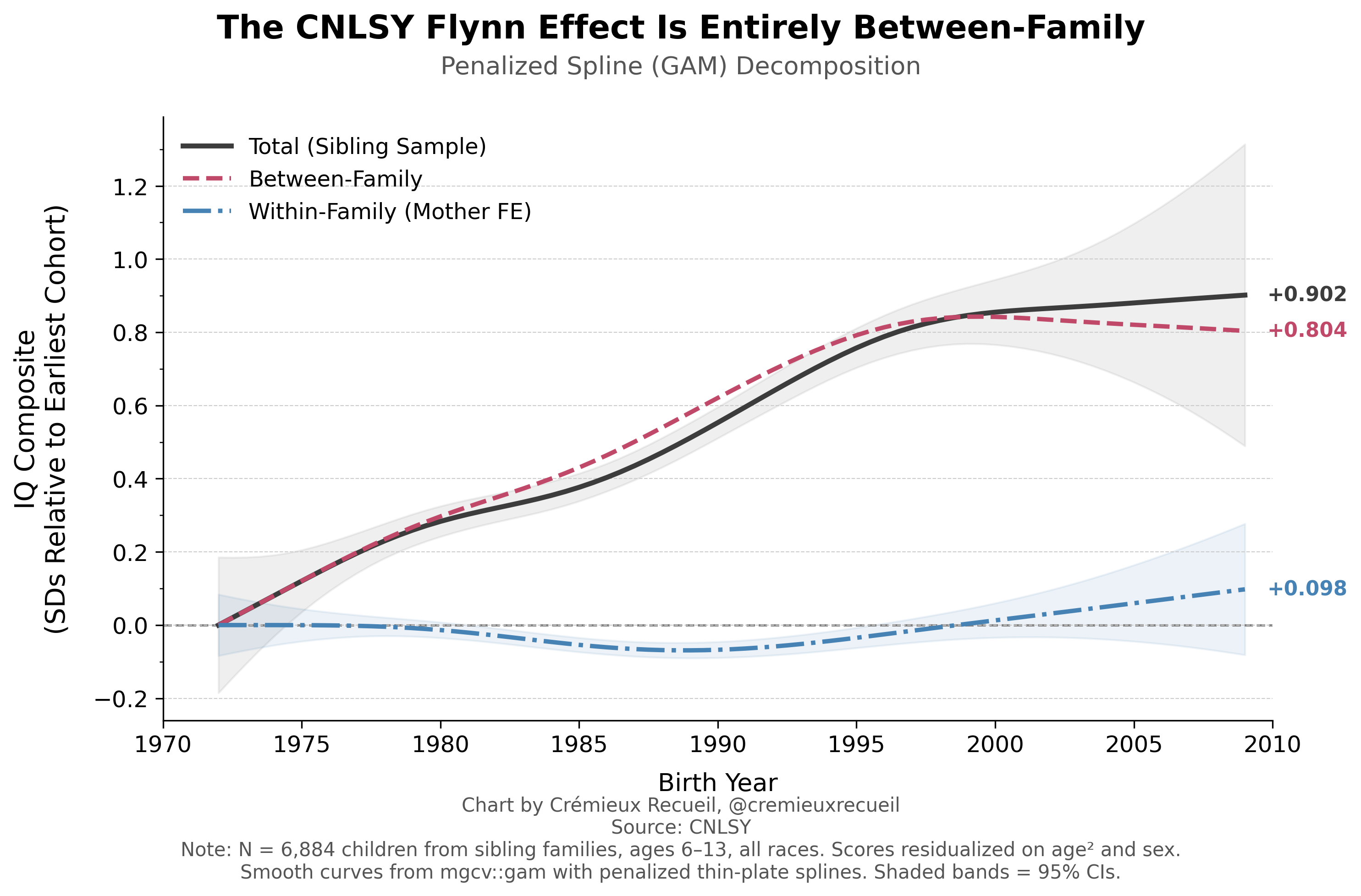
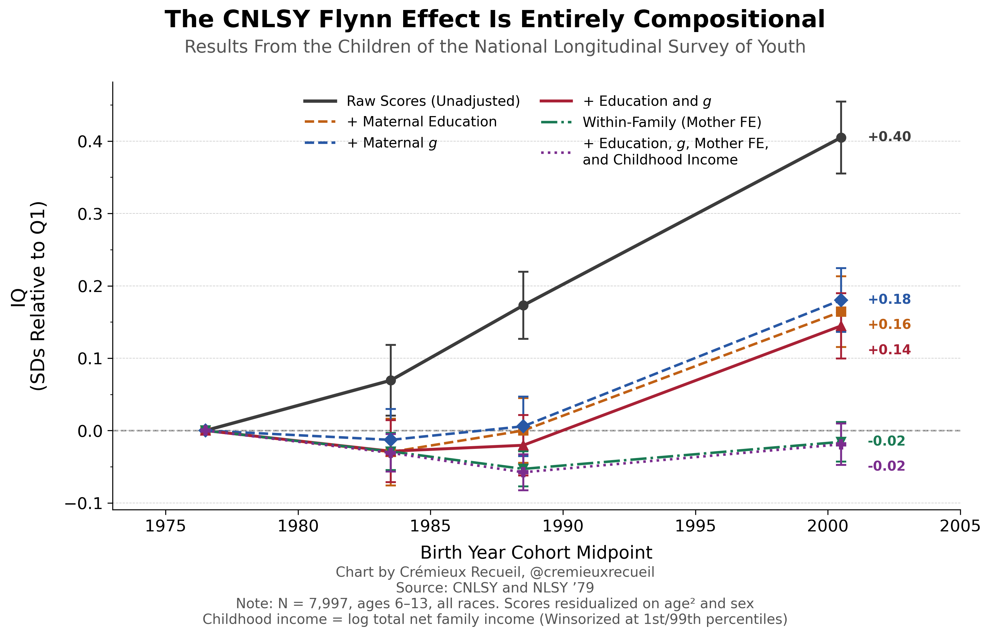
If we take the raw score trend in the CNLSY for kids’ PIAT Mathematics, Reading Recognition, Reading Comprehension, and PPVT performance and we plot it, we can clearly replicate the results obtained by Ang, Rodgers and Wänström. If we control for maternal characteristics relevant to kids’ IQs, such as a mother’s education level and her own intelligence, we can reduce the extent of the “Flynn effect”. But, doing that leaves behind a considerable trend. It’s only when we compare siblings in the same family that we see the effect entirely evaporate. In fact, it goes slightly negative!¹

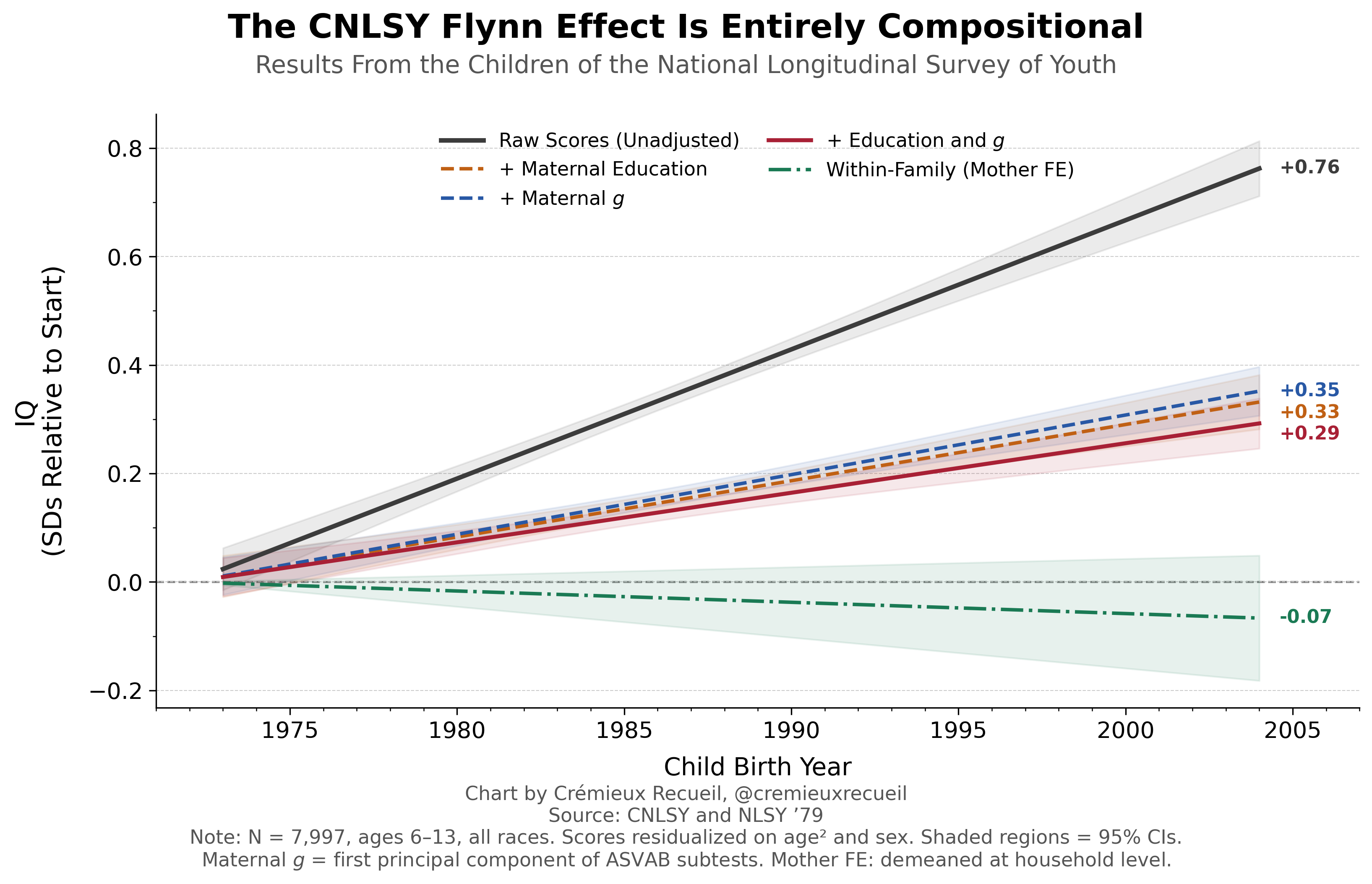
In other words, what Ang, Rodgers and Wänström had dubbed a “Flynn effect” was actually just a compositional effect. We just couldn’t see that this was the case until we controlled away all the confounding characteristics that led to later births also being smarter births. The Flynn effect in the CNLSY was much like the effect of breastfeeding, where it also dissipates within families but it won’t fully disappear if you just throw a handful of the most obvious maternal characteristic controls at it. If you already grok that example, this style of chart might be familiar to you:

Here we have two Flynn effects, both conflated wildly in the literature, and yet totally distinct in character. The Flynn effect in the CNLSY is generated by following a cohort of mothers sampled at different points in their fertile window and noticing a compositional within-cohort selection on who reproduces when. The actual (anti-)Flynn effect, as opposed to this compositional effect, is when you have representative snapshots of the population at a given point in time, and the later group scores better (worse).

If you compared two test norming samples 25 years apart, you would theoretically be looking at two random draws from the population separated only by time, and any compositional changes would be real compositional changes, rather than selection into childbirth. But in the CNLSY analysis, it’s not about a sequence of representative samples, it concerns the children of a single birth cohort, and the older mothers just happened to be better off in many ways that led to a selection-driven false Flynn effect.

In my big article on the Flynn effect and its peculiar inconsistencies, I mentioned another sample that was quite like this. Oberleiter et al. claimed to find a large (~5-IQ point), measurement invariant anti-Flynn effect—that is, real declining ability—in Germany over a brief ten year period (2012-22).

Subscriber Preview: Taking the Flynn Effect Seriously

The issues with this result were two-fold. First, their result was not, in fact, measurement invariant. Maybe that’s enough to disqualify it entirely; we can’t know without the study’s data. Second, there were changes in the underlying population being covered in their comparisons. Their results were based on comparisons of three large, population-representative cohorts of secondary school students, but in this period, secondary school attendance became much less selective and Germany’s young demographics meaningfully changed in that period, too.

The question I asked when I first discussed Oberleiter et al.’s study was whether it was more believable that German kids became one-third of a standard deviation dumber in ten years or that there were sampling issues like we just saw above in the CNLSY. I lean towards thinking that the explanation is more likely the latter.

That study has precedent, too. An earlier study from Germany suggested that a reform that compressed the number of years kids were in school but otherwise maintained the curriculum made German kids a whopping nine IQ points dumber basically overnight. But, this was due to selection. As I showed in my article on it, studies that could account for selection into the sample showed an entirely different result: precise null effects and potentially even small benefits. (My article also covered other negative, sampling-driven results in other countries, like Denmark and the United States.)

Education Isn’t What It Used To Be

---

Yes, This Matters

There are surprisingly many papers out there that conflate ‘the Flynn effect’, as in the psychometric bias-driven change in scores between cohorts, with ‘the Flynn effect’, as in the sampling bias-driven change in scores between select cohorts. These select cohorts can be like subsequent generations of university students—who have become more population-representative as attendance has increased and have accordingly become less elite—or the kids of a birth cohort—where brighter people delay fertility so the kids born later tend to be brighter.

I really wish this were not the case since it misleads people into thinking that there are oftentimes huge and fast population-level changes that just are not so. Alas, that is the sort of thing the public wants: they desire big, flashy results to think deeply about. I’ll repeat my conclusion from my earlier article on the other type of Flynn effect:

People want to think that population intelligence shifts up and down and that people become smarter and dumber all the time, but the reality is that the population practically hasn’t changed any more than you’d predict from shifts in demographics. People want explanations, and they often think they have them, even though most common explanations [for the Flynn effect]—education, technology exposure, family size, hybrid vigor, blood lead levels, genomic imprinting, pathogen levels, nutrition, IQ variability, social multipliers, etc.—cannot be compatible with [its] boring and academic psychometric reality.

The Demise of the Flynn Effect

1. I posted a version of this chart on X/Twitter earlier. In that chart, the within-family result is slightly different because I included controls for birth rank and a superfluous model specification that also included a likely-invalid control in the form of income. Both birth rank and income are invalid due to collinearity.

Within families, birth rank and birth year were far too collinear to separate (r = 0.84). Including birth rank as a control in the within-family model absorbs some 70% of the within-family birth year variance, leaving the Flynn effect identified off of just 8.6% of the original variation. This made for incredibly fragile estimates that were certainly not robust. Without birth rank, the effect is -0.07 SDs (p = 0.26 with OLS and 0.35 with HC5 robust standard errors) and with birth rank, it’s +0.21 SDs (p = 0.047 with OLS and 0.088 with HC5 SEs). If we really want to account for birth order effects, it would be wiser to use an external calibration. If we used the numbers from, e.g., Black et al.’s 20050 Norwegian register data analysis, we would still end up with a nonsignificant result though. And if we went further and did additional robustness tests, the effect would also not stand up to scrutiny. (I’ll get to these below.)

Adding family income to the unadjusted analysis as a control flips the sign to -0.24 SDs and it’s significant, which is an obvious overcorrection. The problem here is that income is mechanically confounded with birth year in the CNLSY. Because the mothers occupy a narrow birth cohort (1957-64), a child’s birth year is almost perfectly determined by maternal age at birth. Income follows a life-cycle pattern where it increases with age through the years that are typically a woman’s full child-bearing years, meaning that later-born children are observed when their mothers are older and typically earning more. This is decidedly not a real intelligence confounder, but rather, it’s the mothers’ age-earnings profile masquerading as a birth year effect and invalidating our birth year-based analysis. Unfortunately—and I checked even though I knew it wouldn’t work—inflation adjustment doesn’t help here because the confound is about the shape of an individuals’ lifetime age-earnings curve rather than nominal price level issues.

The income example is clear, but the issue with birth rank might still feel tougher, because with a very large sample, this shouldn’t be an issue. Unfortunately, we just don’t have a sample large enough. In fact, if we use birth rank, our power is too low to be acceptable to detect reasonably-sized effects. Look at this chart:

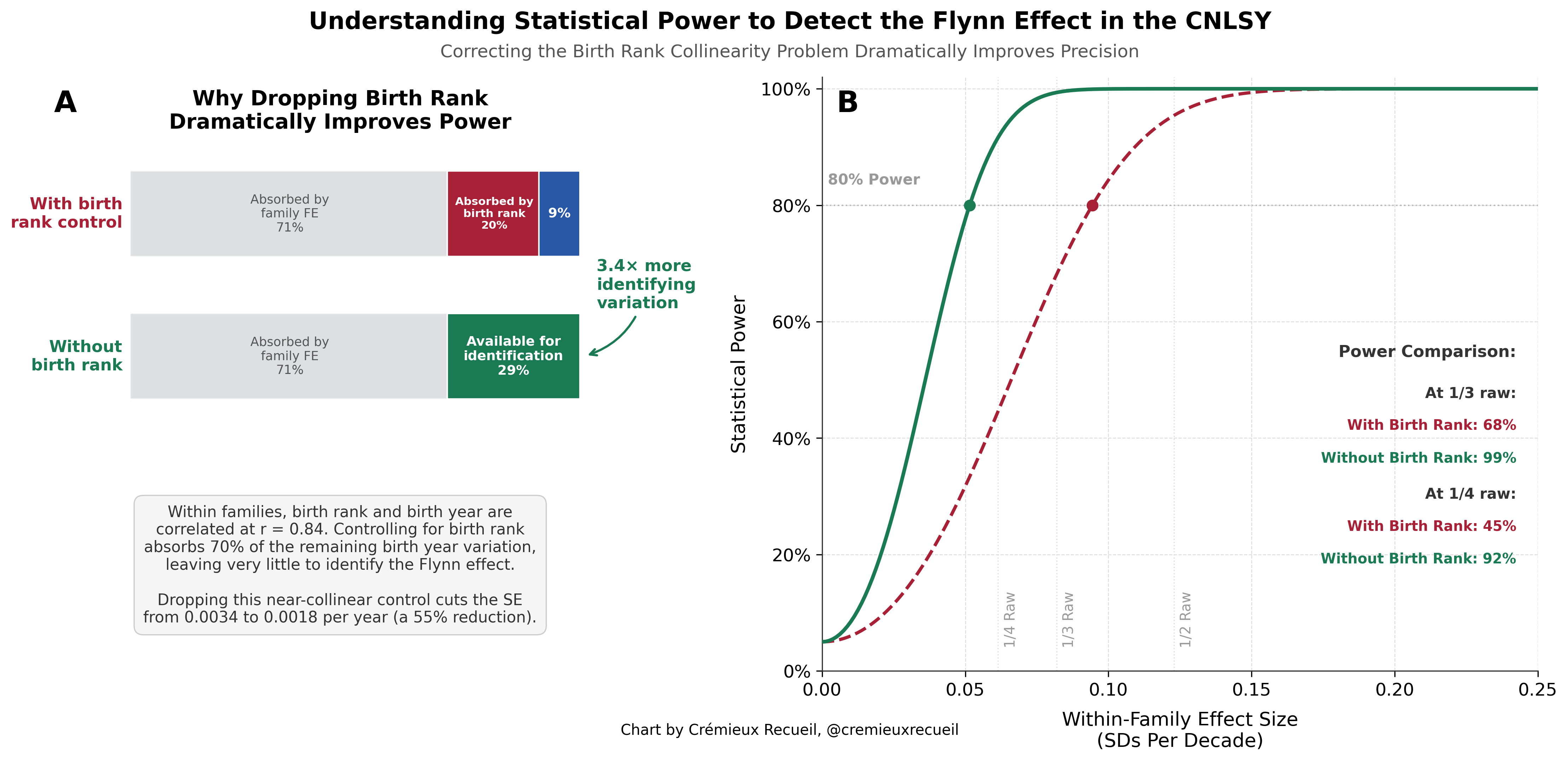
By dropping the birth rank control, we become powered (80%) to detect a Flynn effect that’s roughly one-quarter the size of the typical 3-points-per-decade (~0.75 points) benchmark people tend to cite approvingly. With the birth rank control, we have enough power to detect an effect roughly twice that size. If we recognize the simple fact that birth order effects are (1) not sufficiently large to make much of a different and they’re (2) especially noisy at the ages being looked at here, then we realize there’s even less reason to worry.

Birth Order Effects Needn't Be Biological

Why Accelerated Learning Might Matter More For Larger Families

Now, we should also talk about robustness. In my analysis presented above, I dealt with complete cases for all four of the big ‘IQ tests’ in the battery and I noted the HC5 robust results. If we instead average available cases with three or more tests for a nice, standardized, per-person score composed of as much as we can get, then we gain about 1,000 people (n = 9,009) and the raw result goes to +0.64 SDs, reduces to a similar degree with controls, and becomes -0.02 SDs (p = 0.64) within families. If we use multiple imputation (m = 20), we can get the sample size up to 9,070, achieve the baseline result of +0.65 SDs versus +0.29 SDs with maternal education and g controlled and -0.01 SDs (p = 0.86) within families.

With multiple imputation, the number of test instances available per-person is large enough that a panel model can be used and can meaningfully reduce the size of our standard errors. Thus, we get a maximally large, maximally precise result. The way I do this is multi-step:

1. Demean Y and X at the mother level: composite_dm = composite - mother_mean(composite), birth_year_dm = birth_year - mother(mean(birth_year).

2. Regress: composite_dm ~ birth_year_dm - 1 (intercept-free due to demeaning).

3. Cluster SEs at the child level (i.e., vcovCL(…, cluster = child_id)), since multiple test occasions from the same child are not independent.

4. Apply a degrees-of-freedom correction: sqrt((n-1)/(n-n_families-1))

With the average of 1.57 test occasions per child available with complete cases, the clustering at the child level that’s required to make this work leads to somewhat larger SEs than just using complete cases without attempting to use panel data. With the 3.24 obtained with multiple imputation (harmonic mean k = 2.70), we gain a lot of data, largely for the PPVT, which over half of the kids were missing at some point. This shrinks SEs by ~4% and our final result is +0.01 SDs (SE = 0.00153/year, p = 0.77).

Since Ang, Rodgers and Wänström analyzed only the PIAT Mathematics subtest, I thought I would replicate with their result with single observations, no birth rank control, etc., just to match what they did. In the PIAT Mathematics, the raw trend is +0.83 SDs versus a within-family +0.06 SDs (p = 0.43). For Reading Recognition, the raw trend is +0.71 SDs versus +0.02 SDs within families (p = 0.73). For Reading Comprehension, it’s +0.50 SDs versus -0.15 SDs within families (p = 0.03), which is significant, but is not robust to the methods described above (e.g., HC5 SEs p = 0.053, and other methods lower this more). Finally, for the PPVT, the trend is +0.94 SDs at baseline and -0.15 SDs within families (p = 0.07, and 0.112 with HC5 SEs).

In 2018, Bratsberg and Rogeberg observed that the Flynn effect and its reversal in Norway could be entirely captured within families. I attempted to replicate their result with this data, but due to my smaller sample, my options were more limited. Nevertheless, I used a GAM to check nonlinearity in a manner that’s at least theoretically comparable (in the sense of letting us visualize reversals if they’re present). The test meant taking all sibling pairs (i.e., those with the same mother; yes, I know this is not the same as 50% relatedness, but the results are robust to that, so don’t quibble), taking the residuals, and fitting a penalized spline to those as a function of birth year. By just using the sibling subsample without imputation (result is robust to that), this cuts the sample size a bit, but not meaningfully. Here’s the result:

In other words, I could not replicate their result, but should that have been possible in the first place? It’s possible the trends in Norway and the U.S. in each cohort’s timeframes were not psychometrically alike. Alas, without their data, who can really say?

One other thing I checked was whether the PPVT-R to PPVT-III transition around 2004 affected anything, In principle, that could’ve created an artificial discontinuity in scores if the versions weren’t on the same scale. I don’t think this is an issue for four reasons.

First, there’s no version flag, and I assume the BLS—who maintains the dataset—handled the transition credibly internally. Second, there’s no score discontinuity in 20040. Residualized PPVT scores drift smoothly across the transition, going up by +2.1 in 2002, +2.9 in 2004, and +4.3 in 2006. No jump at 2004 as you might expect. Third, raw score changes are consistent across 2002-2006 and the 19% of children who first enter the sample in 2004 track the pre-2004 trend rather than jumping to some other level. And finally, I checked!

As noted above, the PPVT all-waves result was -0.15 SDs with HC5 p = 0.11. Pre-2004, it’s -0.24 SDs with HC5 p = 0.004, so it does get stronger, but it’s still quite different from the raw result, the difference from which is what I was concerned about. A 4-test composite with PPVT pre-2004 yields -0.28 SDs with HC5 p = 0.0007, and a 3-test PIAT composite yields -0.01 SDs with HC5 p = 0.88. With multiple imputation and child clustering as above, the all-waves result goes to -0.20 SDs (p = 0.016), the pre-2004 result goes to -0.31 SDs, compared to the 4-test PPVT pre-2004 result becoming -0.33 SDs, and the 3-test PIAT becoming +0.01 SDs, with significance and non-significance maintained.

As you can see with the GAM results, there’s a dip in the within-family results that goes away. I’m not sure why. This also replicates in quartile-binned results:

It doesn’t matter, but I would like to know why this is, and though we can’t credibly test it, I think the answer might be birth order, which we dropped for reasons explained above. When we add it back, the PPVT pre-2004 -0.24 SD result goes to +0.07 SDs (p = 0.65) and it’s similar for the other specifications. This might be due to birth order effects being larger for verbal/vocabulary measures than on achievement tests, as is often reported in the literature. The PPVT is a receptive vocabulary test, after all. But as noted above, for reasons of power, this is hard to look into, and very likely to be beyond our means with the present sample.

As a final note, the cross-sectional CNLSY results are more extreme in a latent variable model, and the differences between kids born in different birth year quartiles or just later and earlier years were mostly measurement invariant. But, factor score-based results were still nil within families. Measurement invariance was achievable, because nothing really changed.